Compressor
Introduction🔗
A compressor is a mechanical device which increases the pressure of a gas by reducing its volume. They are commonly used in HVAC&R cycle systems to (nearly) isentropically increase the pressure of the working fluid. There is a wide range of different compressor types and sizes depending on the working fluid (R1234yf, R600a etc.) and the physical conditions dictated by the end application. Accordingly, there is a whole range of manufacturers, who provide performance maps for their compressors. On top of that, there is a whole range of different data sheet formats for compressors, since there is no globally accepted standard on how to test the performance and how to document the performance map. One notable testing standard is the ASHRAE Standard 23, referenced in AHRI standard 540, 2020 Performance Rating of Positive Displacement Refrigerant Compressors.
Similarly, there are different approaches to implement a compressor model in Modelica. Modelon has implemented several compressor models to cover a range of different end applications and required inputs for successful parametrization.
One implementation uses table-based efficiency maps dependent on compressor speed and pressure ratio, as the ratio of absolute discharge pressure divided by absolute suction pressure. This implementation can be used for a given performance map from a compressor data sheet, e.g. according to the ASHRAE standard. Conversion to the right parameters might be required, depending on the data sheet.
Another implementation uses the 10-coefficients characteristic map, based on the AHRI Standard 540, 2020. This implementation can be used if the ten coefficients for the compressor characteristics are given.
You can find compressor models in our Modelon Base Library, Air Conditioning Library, Engine Dynamics Library, Environmental Control Library, Jet Propulsion Library, Pneumatics Library, Vapor Cycle Library, as well as a liquid compressor in the Thermal Power Library.
This tutorial aims to explain the basic implementation of the compressor models that are part of Vapor Cycle Library (VCL), and how to parametrize a VCL compressor model with ASHRAE data as starting point, the general procedure to parametrize a compressor with non-standardized compressor performance data sheets, and the parametrization using the ten coefficients implementation.
This skill is important if you will be modeling using commercially available compressors.
It is recommended to have some understanding of thermodynamics for this tutorial.
This tutorial is divided into an Implementation section that will explain the underlying implementation, and Parametrization section that will give step-by-step instructions on how to parametrize the compressor models. Each section is sub-divided into a section for the table-based efficiency map implementation containing an ASHRAE example and a generic example, and the ten-coefficients implementation with a generic example. Depending on your compressor data at hand, the irrelevant implementation and parametrization subsection can be skipped.
You will need approximately 30 minutes to finish the ASHRAE example tutorial.
Implementation🔗
Table-based efficiency map🔗
The efficiency map implementation uses three efficiencies to map the compressor characteristics: The volumetric efficiency \(\eta_{vol}\), the isentropic efficiency \(\eta_{isen}\), and the mechanical efficiency \(\eta_{mech}\). All of these can vary for different mass flows \(\dot{m}\), relative displacement, and pressure ratios \(p_{ratio}\) as the ratio of absolute discharge pressure \(p_{dis}\) over absolute suction pressure \(p_{suc}\). The three efficiencies are defined as:
with \(ρ\) as density of the working fluid on the suction side, \(V_d\) as displacement volume, \(N\) as compressor speed (in rps), \(h\) as the corresponding specific enthalpy, and \(P_{shaft}\) as the power crossing the mechanical flange. By variable separation, we can re-formulate the equations to get
with \(x\) as the relative displacement. These six functions can be described by six corresponding tables. This is the basic implementation that is used in the VCL model VarDisplacementTableBased. For many applications, a compressor with a fixed displacement is used. In that case, the terms \(g\) dependent on relative displacement \(x\) in Eq. 4 -6 can be set to 1. An implementation of a corresponding compressor model can be found in the VCL model FixedDisplacementTableBased. Manufacturer data typically needs to be converted into this format. For this matter, the VCL model EvaluateEfficiencies can be used. The general procedure is described in section Parametrization.
As mentioned above, one common way of testing compressors is according to the ASHRAE Standard 23. The provided test data will be power input, refrigerating capacity and mass flow rate as a function of condensing and evaporation temperature. This is not in the format of efficiency maps. However, the VCL compressor model FixedDisplacementTableBased_ASHRAE uses the power, capacity and mass flow rate maps as input and converts it automatically into the format of efficiency maps. In section Parametrization, the correct usage of the model is explained.
Ten coefficients🔗
The ten coefficients implementation uses 10 regression coefficients provided by the manufacturer. The underlying base equation is
with \(X\) as refrigerating capacity, power input, or refrigerant mass flow rate, \(T_{dis}\) as discharge point temperature, \(T_{suc}\) as suction point temperature, and \(C_1\) through \(C_{10}\) as regression coefficients provided by the manufacturer for refrigerating capacity, power input, and refrigerant mass flow rate respectively.
One set of coefficients corresponds to the characteristics of one compressor speed. If several compressor speeds are of interest, one set for each speed has to be provided.
The VCL compressor model TenCoefficientsBased uses the ten-coefficients approach to model the compressor. In this model, the parameter \(C\) corresponds to the 10 coefficients for refrigerating capacity, \(P\) corresponds to the 10 coefficients for input power, and \(F\) corresponds to the 10 coefficients for mass flow rate. The parameter \(S\) is the compressor speed in Hz at which one set of coefficients is valid.
Parametrization🔗
Preparation🔗
All approaches described in this section will be tested with the same base model. Let us set up the right workspace configuration for that. The compressor parametrization in this tutorial requires to have Modelon Impact Pro license, which includes all Modelon libraries. The ![]() Vapor Cycle Library will be used in this workshop.
Vapor Cycle Library will be used in this workshop.
The instructions are valid for Modelon Impact on cloud.
- Run Modelon Impact.
- Create a new workspace called Tutorials.
- Create a new Project called Compressor_testing.
- In the new project, create a new Package by clicking the "+" symbol. Call the package Compressor_test
- Navigate to VaporCycle.Compressors.Experiments.TestBench, right-click the model and select "Extend..." to extend the model to your project. Call the model Compressor_Test.
We are now ready to go through the parametrization process.
Table-based efficiency map🔗
By going through this section, you will learn how to parametrize compressor models from manufacturer data sheets.
When working with tables as parameter, there are typically two ways in our libraries to input the data into a model:
- Input from a formatted file.
- Direct input of table values separated by specific symbols.
Your compressor data is typically provided by the supplier in the form of a table or a plot.
In this subsection, we will go through an example on how to parametrize the compressor model with tabulated AHSRAE data from file, and a general procedure of how to parametrize a compressor from generic plotted data.
Example: Tabulated ASHRAE data
In this example, we will learn how to correctly format tabulated ASHRAE data to work with our compressor model.
For the parametrization process in this example, we will use compressor data sheet. An Excel sheet containing the extracted data from the manufacturer data sheet can be found in VCL's Resources folder VaporCycle/Resources/Data/compressor/dataASHRAE_example.xlsx.
Before we start with our compressor parametrization, let us set up the testbench. The setup of the testbench should be done according to your end application of the compressor.
- Go into your Workspace.Compressor_TestBench model.
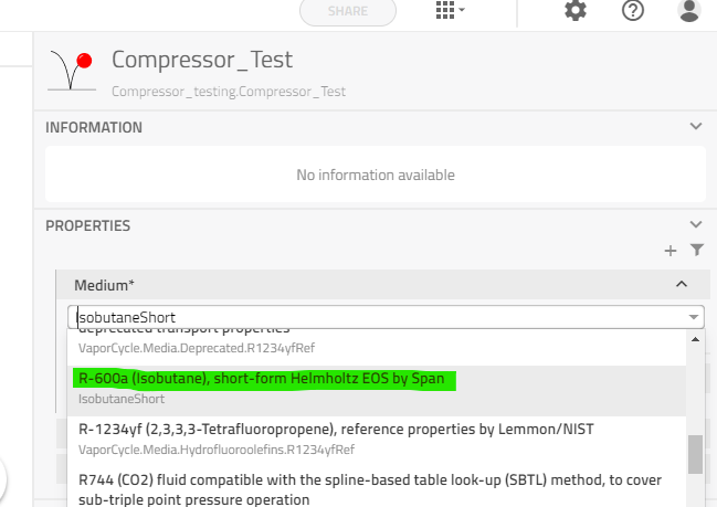
- In the Properties tab, select the Medium that is used with your compressor. In our case it is Isobutane. Select IsobutaneShort as Medium.
- In the compressorData tab in the General sub-tab, set the maximum displacement according to your compressor specifications. Remember to convert it to \(m^3\). In our case, set MaximumDisplacment to \(11.14e-6 m^3\).
- Switch to the Experiment sub-tab and set your experiment conditions.
We will use the conditions as shown in table below:
| Parameter | Value | Unit | Explanation |
|---|---|---|---|
| speed0 | 20 | rps | Compressor speed |
| displacement0 | 1.0 | - | Relative displacement |
| p_in | Medium.saturationPressure_TX(238.15) | Pa | Inlet pressure |
| p_out | Medium.saturationPressure_TX(308.15) | Pa | Outlet pressure |
| T_in | 305.35 | K | Inlet temperature |
We can leave the remaining parameters in the Experiment tab as they are.
This concludes the testbench setup. Let us now look at how to get the ASHRAE data into our compressor model.
One basic file format that can be used in Modelica are txt-files. The data in the txt-file needs to be in a certain format. Look at the example txt-file below:
#1

double table_name1(rows,columns)
Compressor_speed Evap_Temp1 Evap_Temp2 ...
Cond_Temp1 Table1_data22 Table1_data23 ...
Cond_Temp2 Table1_data32 Table1_data33 ...
.
.
.

double table_name2(rows,columns)
Compressor_speed Evap_Temp1 Evap_Temp2 ...
Cond_Temp1 Table2_data22 Table2_data23 ...
Cond_Temp2 Table2_data32 Table2_data33 ...
.
.
.
The first keyword is "double" which describes the data type of the table entries. This is followed by the array name "table_name1" and the array size. The first value in the brackets (i.e. rows) indicates the number of rows, the second value (i.e. columns) indicates the number of columns. In the next line, you can start inserting your data. Each value is delimited by a space. The end of one row is delimited by a line break (Enter). Modelica models can read from these files when given the file name and array name.
Tip
There are other table formats such as mat-files, xml-files, xlsx-files that are supported by access models in the Modelon Base Library. Depending on your data at hand, another format might be easier to use.
Our ASHRAE compressor model dictates a few more requirements on the data format:
- The data set is numbered with #n at the start, with n as your data set number.
- The first value [1,1] of the table (compressor_speed above) is the compressor speed in rps.
- The first column [2:end,1] of the table (Cond_Temp above) is the condensing temperature in K.
- The first row [1,2:end] of the table (Evap_Temp above) is the evaporating temperature in K.
- The rest of the table [2:end,2:end] is the data for the particular parameter: Power in W, capacity in W, mass flow rate in kg/s.
Let us create the tabulated maps that our compressor model uses.
Tip
If you are familiar with Modelon Impact's VSCode environment you can create your compressor characteristics txt-file there.
- On your desktop, create a txt-file and name it "mflow3D.txt".
- Open the file and add "#1" to the first line and go two lines lower.
If we look at the third page of the compressor data sheet (see link above), we can see that for one compressor speed, we have 4 condensing temperatures and 6 evaporating temperatures. We need one extra row and column for headers:
- Write double table_1(5,7).
When we fill in the sheet data, remember to convert to SI units.
-
In the next line, fill the first line of our table with compressor speed (in rps) followed by evaporating temperatures (in K):
20.0 238.15 243.15 248.15 253.15 258.15 263.15
-
In the following line, fill the first value with the condensing temperature (in K) and the remaining six with the mass flow rate (in kg/s) of this condensing temperature:
308.15 1.4444E-04 1.9167E-04 2.5E-04 3.1667E-04 4.0E-04 4.9722E-04
-
Repeat step 10 for the remaining condensing temperatures.
-
Create tables corresponding to the other compressor speeds by repeating step 8 to 11.
The first part of your mflow3D.txt should now look like this:
#1

double table_1(5,7)
20.0 238.15 243.15 248.15 253.15 258.15 263.15
308.15 1.4444E-04 1.9167E-04 2.5000E-04 3.1667E-04 4.0000E-04 4.9722E-04
318.15 1.2778E-04 1.7500E-04 2.3333E-04 3.0000E-04 3.8056E-04 4.7778E-04
328.15 1.1667E-04 1.6389E-04 2.1667E-04 2.8333E-04 3.6389E-04 4.6111E-04
338.15 1.0833E-04 1.5278E-04 2.0556E-04 2.6944E-04 3.4722E-04 4.4167E-04

double table_2(5,7)
33.333333333333336 238.15 243.15 248.15 253.15 258.15 263.15
308.15 2.4444E-04 3.0278E-04 3.8889E-04 5.0278E-04 6.4444E-04 8.1389E-04
318.15 2.1667E-04 2.8056E-04 3.7500E-04 4.9722E-04 6.5000E-04 8.3333E-04
328.15 1.7222E-04 2.3611E-04 3.2778E-04 4.5556E-04 6.1389E-04 8.0556E-04
338.15 1.8333E-04 2.4167E-04 3.3056E-04 4.5556E-04 6.1389E-04 8.0833E-04
The last two tables are not shown here.
-
Save and close this file.
-
Repeat step 6. to 13. for the refrigerating capacity and power. Call the txt-files "capacity3D.txt" and "power3D.txt" respectively.
You should now have three files containing 4 tables each.
Note
You can find the three txt-files for this example in the Resources folder of VCL: VaporCycle/Resources/Data/compressor.
We can now import our three compressor maps to our Modelon Impact project.
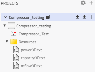
- Select the three txt-files and upload them to the Resources folder of your project through drag-and-drop.
Your project should now look like this:
We can now finalize the compressor parametrization.
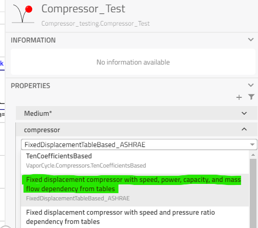
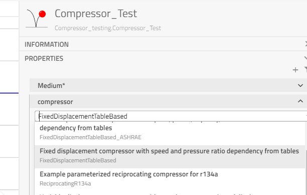
- In your Compressor_Test model, navigate to compressor sub-tab.
- In the compressor sub-tab, select FixedDisplacementTableBased_ASHRAE from the drop-down menu.
- In the compressor model, switch to Table data tab.
- In the Medium_tables, select IsobutaneShort as medium model.
We can now proceed to load in our previously created txt-files. We will use the Modelica Standard Library model Modelica.Utilities.Files.loadResource.
- Right click on your power3D.txt file in the Resources folder and select "Copy path" to copy the path to the file.
- In the compressor's Table data tab, insert Modelica.Utilities.Files.loadResource("modelica://Compressor_testing/Resources/power3D.txt").
- Repeat step 5 and 6 for the capacity and mass flow rate.
Tip
You can drag-and-drop the txt-file into your model's text field and Modelon Impact will automatically fill in the field with the correct function call, i.e. Modelica.Utilities.Files.loadResource("modelica://Path/To/Your/Text-file.txt").
Your model is now ready to run. Click the run button to get an overview of your results.
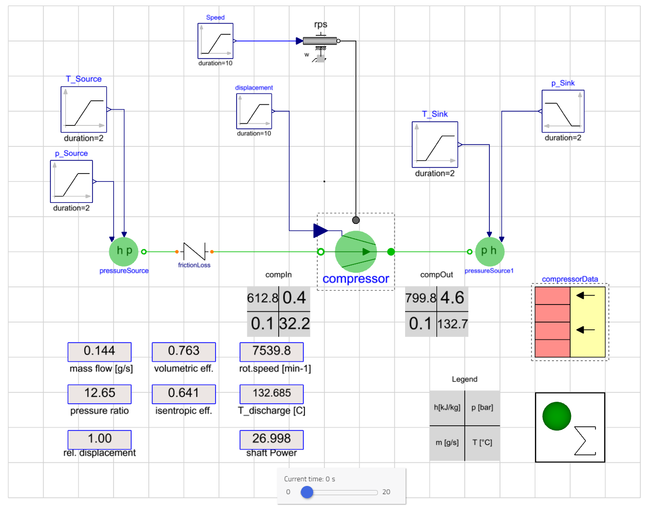
This concludes the tutorial of this example.
Procedure for generic, plotted data
In this sub-section, we will go through the general procedure on how to format generic, plotted compressor map data and convert to efficiency maps to work with our compressor model. We will assume that the compressor has a fixed displacement. This procedure is incomplete as there are steps that highly depend on the format of the supplied data.
This example will use a few external tools. An explanation of the usage of the external tools is not part of this tutorial.
We first need to digitize our data. Ideally, we can use the digitzed data to do some automated calculations (e.g. in Excel). For tabulated compressor data, we can just use the values directly. If the compressor map is plotted, we need to convert the plot into table data. There are external tools that can help you with this, e.g. Engauge Digitizer or WebPlotDigitizer. A general procedure looks like this:
- Digitize the plotted/tabulated data.
- For digitization from plotted data: Plot the extracted data and compare with the original plot to verify that it was digitized correctly.
- Convert your data to SI base units.
This can be done in Excel with the right conversion factors.
Depending on your data, you now have two options on how to proceed: You can either convert your data to
- the three efficiencies (see Eq. 1-3), or to
- performance maps according to the ASHRAE standard.
In case 2, you can then continue with the example parametrization in the previous sub-section. Here, we will pursue case 1.
With the digitized data, we need to find the dependency of the compressor speed and pressure ratio (of absolute pressures) against the efficiencies, or variables that describe the efficiency. For the volumetric efficiency,
we have a direct dependency with the compressor speed \(N\). Typically, the mass flow rate \(\dot{m}\) is dependent on pressure ratio and compressor speed.
- Convert your digitized data to get a mass flow rate map over pressure ratio and compressor speed.
Ideally, we want all our variables (especially the efficiencies) that are dependent on pressure ratio and compressor speed in the following table format:
This will simplify the model input process later on.
From Eq. 1, suction side density and displacement volume are constant parameters. Often, you do not get the suction side density as data from the supplier. Instead, they might give you the measurement conditions as a pair of pressure and temperature, or saturation pressure, or saturation pressure and superheat. Double-check with your supplier under which conditions the data was created. From the provided conditions, you can then calculate/look up the density with tools like RefProp or CoolProp. These tools have tabulated data for a range of media around the two-phase region.
- Look up the media density at the experiment conditions.
- Calculate the volumetric efficiency map.
Next, let us look at the mechanical efficiency:
We have already calculated the mass flow rate. As explained earlier, we can get the fluid properties on the suction side through tools like RefProp. Here, we can also find the enthalpy on the suction side. Typically, we can look this up by using the suction side vapor saturation temperature (+ superheat temperature if given). The shaft power is typically provided in some form of mapped data. Currently, there is no universal standard for compressor suppliers to map their data, which makes the next step vague:
- Calculate the shaft power map.
Depending on the provided supplier data, the steps to get the shaft power vary and need to be carried out individually. At this point, we can not provide a universal guide.
Now, we need the value of one more variable. If you get data on the fluid properties on the discharge side, you can look up the discharge enthalpy and then calculate the mechanical efficiency. However, it is also possible that the mechanical efficiency is provided (possibly through conversion of data). In that case, we can use the efficiency to calculate the discharge enthalpy (we will need it in the next step).
-
a) Look up the discharge enthalpy for the given experimental data.
b) Convert your digitized data to get a mechanical efficiency map over pressure ratio and compressor speed. -
a) Calculate the mechanical efficiency map.
b) Calculate the discharge enthalpy map.
Finally, let us look at the isentropic efficiency:
We already have the suction and discharge enthalpy from the previous steps. We can get the isentropic enthalpy through a table-lookup. The ideal compressor increases the pressure of the working fluid isentropically. We know the suction pressure and suction enthalpy. With this, we can look up the corresponding entropy. Using the discharge pressure (or pressure ratio) together with the constant entropy, we get the ideal thermodynamic state after compression. We can then look up the enthalpy of this thermodynamic state.
- Look up the isentropic enthalpy, that you get for an isentropic pressure increase.
- Calculate the isentropic efficiency map.
We now have all the data together and can start parametrizing our compressor model.
- Go into your Workspace.Compressor_TestBench model.
- In the Properties tab, select the Medium that is used with your compressor.
- In the compressorData tab in the General sub-tab, set the maximum displacement according to your compressor specifications. Remember to convert it to \(m^3\).
- Switch to the Experiment sub-tab and set your experiment conditions. This can be done according to your end application conditions. Remember to convert units if necessary.
- Navigate to compressor sub-tab.
- In the compressor sub-tab, select FixedDisplacementTableBased from the drop-down menu.
- In the compressor model, switch to Table data tab.
- Take away the tick from tableOnFile (i.e. set to False).
In volEffMap, etaIsMap and etaMechMap, we need to put in our map data. As mentioned above, for our model to work, we need the characteristic maps in the following table format:
Tip
This is the standard table format for our VCL models that use efficiency maps, such as FixedDisplacementTableBased and VarDisplacementTableBased. For models that use ASHRAE data as input, the format is different. You can read about it in example 1.
The Modelica syntax for a generic table is:
[Cell_11, Cell_21, Cell_31, ..., Cell_n1; Cell_21, Cell_22, Cell23, ..., Cell_2n; ...; Cell_n1, ..., Cell_nn]
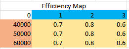
The table starts with '[' and ends with ']', each cell value is delimited by a comma , and each line break is delimited by a semicolon ;. The format explaining table figure from above (Efficiency Map) would translate to:
[0, 1, 2, 3; 40000, 0.7, 0.8, 0.6; 50000, 0.7, 0.8, 0.6; 60000, 0.7, 0.8, 0.6]
- In the field volEffMap, put in the calculated volumetric efficiency map following the above format.
Tip
If you have your efficiency maps in the right format in Excel, you can instead use Modelon Impact's Copy/Paste function for Excel tables.
- Repeat step 9 for the isentropic efficiency in etaIsMap, and the mechanical efficiency in etaMechMap.
Your model is now ready to run. Click the run button to get an overview of your results.
This concludes the tutorial of this general example.
Ten coefficients🔗
By going through this section, you will learn how to parametrize compressor models using manufacturer provided ten coefficients.
As the ten-coefficients method was made for single speed parametrization, we will only parametrize for a single speed.
- Go into your Workspace.Compressor_TestBench model.
- In the Properties tab, select the Medium that is used with your compressor.
- In the compressorData tab in the General sub-tab, set the maximum displacement according to your compressor specifications. Remember to convert it to \(m^3\).
- Switch to the Experiment sub-tab and set your experiment conditions. This can be done according to your end application conditions. Remember to convert units if necessary.
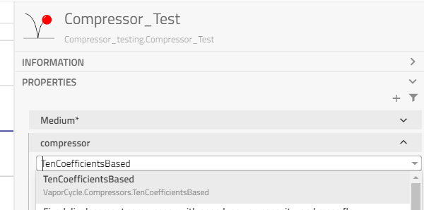
- Navigate to compressor sub-tab.
- In the compressor sub-tab, select TenCoefficientsBased from the drop-down menu.
- In eta_Mech, set the mechanical efficiency as provided by the manufacturer. It is typically a value between 0.9 and 1.
- In S, enter the compressor speed in Hz for which the ten coefficients apply. Put the value in '{}'.
- In coefficients_units, select the unit (SI or imperial) in which your coefficients are provided.
- In C, enter the coefficients for the refrigerating capacity.
- In P, enter the coefficients for the input power.
- In F, enter the coefficients for the mass flow rate.
Your model is now ready to run. Click the run button to get an overview of your results.
This concludes the tutorial of this general ten coefficients example.
Congratulations! You have now made your first steps to become a compressor modelling expert.