Bag Filter🔗
Outline🔗
-
Introduction
-
Plant Introduction
-
System Layout
-
System Components
-
System Overview
-
Component Parameterization and Properties
-
Simulation and Results
Purpose🔗
This is a step-by-step tutorial to learn how to work with a catalytic bag filter model that treats flue gas emissions from combustion plants in Modelon Impact.
-
This tutorial is modeled primarily using components from the Thermal Power Library and Modelica Standard Library.
-
The tutorial goes over component by component modeling and parametrization and explains how the flow of species happens inside the system.
-
After this tutorial, you will be able to enter the inputs into the model based on the data you have and generate results.
-
The focus of this tutorial will be to familiarize yourself with the relevant components and how they function.
-
The tutorial will not show how the components themselves are modeled. This requires a different level of understanding of physics. If interested, go to the code layer for those components.
Related articles🔗
Requirements and Pre-requisites🔗
-
Duration: 90 minutes.
-
Access to the “FlueGasTreatment” package.
Downloads🔗
“FlueGasTreatment” package (.zip file) has to be imported in the workspace to simulate this tutorial.
Plant Introduction🔗
-
The flue gas treatment plant intakes flue gas and treats the gaseous pollutants (namely HCl and SO2) using a bag filter.
-
The bag filter uses a Shrinking Core Model that describes the amount of gaseous pollutant that is being captured by a particle of a given size while the unreacted core is shrinking.
-
The sorbent used here is limewater.
-
Once the pollutants are settled, the ash from the flue gas is removed using an electrostatic precipitator. At the end of the simulation, we calculate the concentration of HCl and SO2 removed and the required flow rate of limewater to neutralize these pollutants.
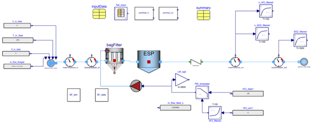
System Layout🔗
The plant to be modeled is present in FlueGasTreatment.Tests.BagFilter_LW_SO2HCl. Below, you’ll see the plant schematics in Impact including the closed-loop controllers that are required to control the limewater flow rate inside the bag filter.
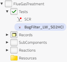
System Components🔗
The FlueGasTreatment package consists of the following sub-packages:
-
The test bench in the “Tests” package, contains the bag filter model. This model consists of different records/data taken from “Records” package. Our model naturally contains different components which are taken from “Subcomponents” package. Furthermore, the reactions which are used in the modeling of these components are taken from “Reactions” package. You can find the path of all the components used in the bag filter model below. If you need to learn more about these components, you can go to the information section for these components by going to these paths.
-
BagFilter_LW_SO2HCl comprises different components like BagFilter and ESP etc. which are taken from the SubComponents sub-package:
i. bagFilter: FlueGasTreatment.SubComponents.BagFilter.BagFilter_NaHCO3_SO2_HCl
ii. ESP: FlueGasTreatment.SubComponents.ESP
iii. sorbentSource: FlueGasTreatment.SubComponents.SorbentSource
iv. SF_sim: FlueGasTreatment.SubComponents.StoechiometryCoefficient
v. SF_data: FlueGasTreatment.SubComponents.StoechiometryCoefficient
-
Other components are taken from the Records sub-package:
i. plantData_in: FlueGasTreatment.Records.InputData
ii. plantData_out: FlueGasTreatment.Records.InputData
-
Components taken from Thermal Power Library:
i. flowsource_track_mass1: ThermalPower.FlueGasTreatment.Sources.Flowsource_mass_traces
ii. frictionLoss1: ThermalPower.FlueGas.FlowResistances.FrictionLoss
iii. reservoir_mass_traces: ThermalPower.FlueGasTreatment.Sources.Reservoir_mass_traces
iv. molarFlowSensor_in: ThermalPower.SeparationProcess.Sensors.MolarFlowSensor
v. concentration_in: ThermalPower.SeparationProcess.Sensors.ConcentrationSensor
vi. molarFlowSensor_out: ThermalPower.SeparationProcess.Sensors.MolarFlowSensor
vii. concentration_out: ThermalPower.SeparationProcess.Sensors.ConcentrationSensor
viii. inputData: ThermalPower.FlueGasTreatment.Records.Data.InputData_BagReactor
ix. summary: ThermalPower.FlueGasTreatment.Records.Data.Summary_filter
-
Components taken from Modelica Standard Library:
i. Tab_input: Modelica.Blocks.Sources.CombiTimeTable
ii. C_in_data: Modelica.Blocks.Sources.RealExpression
iii. T_in_data: Modelica.Blocks.Sources.RealExpression
iv. X_in_data: Modelica.Blocks.Sources.RealExpression
v. m_flow_fluegas: Modelica.Blocks.Sources.RealExpression
vi. m_flow_feed_s: Modelica.Blocks.Sources.RealExpression
vii. HCl_data1: Modelica.Blocks.Sources.RealExpression
viii. HCl_sim1: Modelica.Blocks.Sources.RealExpression
ix. LW_kgh: Modelica.Blocks.Math.Gain
x. PID_limewater: Modelica.Blocks.Continuous.LimPID
xi. HCl_filtered: Modelica.Blocks.Continuous.FirstOrder
xii. n_HCl_filtered: Modelica.Blocks.Continuous.FirstOrder
xiii. n_SO2_filtered: Modelica.Blocks.Continuous.FirstOrder
xiv. SO2_filtered: Modelica.Blocks.Continuous.FirstOrder
System Overview🔗
This section describes how the flue gas flows in the overall system through different components.
-
The flue gases are used as a flow source in the system. The concentration of species, temperature, gas composition and mass flow rate of the flue gas are specified as inputs to the system.
-
Limewater is used as a sorbent source in the system. Mass flow rate of limewater (Ca(OH)2) is determined based on the concentration of HCl in the flow source using a PID control system. PID controller uses only the concentration of HCl as an input because the concentration of HCl is much greater than the concentration of SO2.
- The flue gases are passed through the bag filter where the pollutants (SO2 and HCl) are neutralized by the limewater which is entering through the sorbent source. Here, these two pollutants are getting separated from the flue gas. Then flue gas goes to the electrostatic precipitator where dust/ash is deposited.
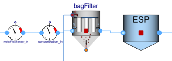
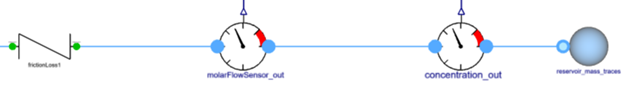
- Flue gas is now passed through a flow resistance which results in a pressure drop and then it reaches a sink which is maintained at a constant pressure and temperature.
Component Parameterization and Properties🔗
This section defines each component in detail in terms of parameterization, properties, and reactions (if needed).
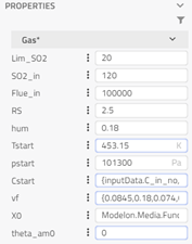
- inputData: This block is used as a record for storing some constant parameters like target SO2 concentration, start pressure value, etc.
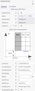
- Tab_input: This table contains values of the following properties wrt time: HCl in, SO2 in, NO in, O2 in, Treactor in, Tfilter in, dpfilter, HCl out, SO2 out, O2 out, H2O out, NH3 out, NO out, ash out, Vfluegas, T out. ‘In’ refers to the inlet and ‘out’ refers to the outlet condition in the plant. If the values are unknown, we write -1000 (or any negative value) in the table. Linear interpolation is done to obtain values at a given time. The concentration values are provided in mg/Nm3 (dry at 11% O2).
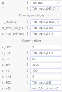
- plantData_in: We specify the inlet concentration of species from the Tab_input table and we also specify some other constants for plant inlet. This block is used to convert concentrations in mg/Nm3 (dry at 11% O2) to SI units.
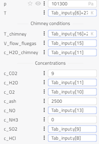
- plantData_out: We specify the outlet concentration of species from the Tab_input table and we also specify some other constants for plant outlet. This block is used to convert concentrations in mg/Nm3 (dry at 11% O2) to SI units.
-
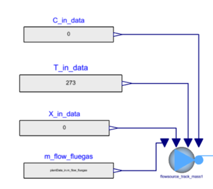
C_in_data: Concentration of trace gas species is provided in the order of (NO, NH3, SO2, HCl). Since they are trace in quantity, they don’t affect the fluid properties and don’t add up to 1.
-
T_in_data: The temperature of flue gas at the inlet is specified in this expression.
-
X_in data: Gas composition (mass fraction) in the order of (CO2, H2O, O2, N2, Ash) is provided. They all add up to 1 and affect the bulk fluid properties. This mass fraction is specified to compute the density, specific heat capacity etc. of the mixture using the properties from Modelon Base Library.
- Ideal gas behavior is assumed in this model.
-
m_flow_fluegas: The mass flow rate of flue gas is specified in this expression.
-
flowsource_track_mass1: Flow source specification of flue gas is defined in this component using inputData and concentration, temperature, mass fraction and mass flow rate of flue gases using the connectors. This sets the mass flow and temperature boundary conditions for our gases in the system at the plant inlet.
-
molarFlowSensor_in and molarFlowSensor_out: This sensor converts mass flow rate in kg/s to mol/s. The molar flow rate is used to compute stoichiometry factors for the species.
-
concentration_in and concentration_out: This sensor converts concentration in kg/s to mg/Nm3.
-
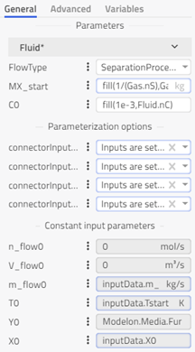
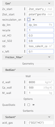
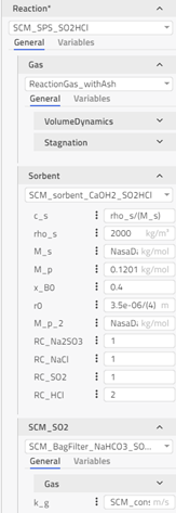
bagFilter: The bag filter with shrinking core describes the acids’ neutralization (HCl, SO2) with the sorbent of Ca(OH)2. All particles of a given reactant, including in the REFIOM stream, will be assumed to have the same outer diameter. The different conversion rates of the reactant inside the particles are accounted for. Modeling approach, equations and assumptions for this component can be found in the information section of the component in FlueGasTreatment.SubComponents.BagFilter.BagFilter_NaHCO3_SO2_HCl. Different options in the drop-down menu can be chosen in the reaction tab based on which gas, sorbent, SO2 or HCl properties we want to use. This will decide the values of different constants and coefficients.
-
ESP: Electrostatic precipitator is used to capture of dust particles in the flue gas, and predict impact of voltage, mass flow and dust concentration (No power electronics). The ESP efficiency, i.e. the mass flow rate ratio between collected particles and incoming particles will be computed as an explicit function of the total collecting area, the gas flowrate and the energizing voltage applied to the electrodes. Assumptions, main equations, and references for this component can be found in the information section of the component in ThermalPower.FlueGasTreatment.ESP.ESP_ash.
-
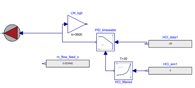
sorbentSource: This component is passing on the value of sorbent (limewater) flow rate to the bagFilter.
-
HCl_sim1: Measurement concentration of HCl is specified in this expression for the PID controller to vary the feed rate of the sorbent.
-
HCl_data1: Setpoint for HCl target concentration
-
HCl_filtered: This block adds time delay to the measurement of HCl concentration. Since the concentration of HCl is fluctuating a lot, their derivative terms might tend to infinite at certain points, hence to smoothen these output values, these filtering mechanisms are involved.
-
PID_limewater: PID controller uses HCl_sim1 and HCl_data1 to determine the appropriate sorbent feed rate into the sorbentSource.
-
frictionLoss1: This component adds a generic flow resistance to create a pressure drop in the flue gases.
-
reservoir_mass_traces: This sink is maintained at a fixed temperature and pressure boundary conditions. It means it has an infinite capacity to store trace gases.
-
n_HCl_filtered, n_SO2_filtered and SO2_filtered: It gives us the outlet concentrations of HCl (in molar), SO2 (in molar) and SO2 (in mg/Nm3) after a time delay. Since the concentration of SO2 and HCl is fluctuating a lot, their derivative terms might tend to infinite at certain points, to smoothen these concentrations, these filtering mechanisms are applied.
-
m_flow_feed_s: Mass flow rate of the feed (limewater) in kg/s.
-
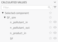
SF_sim: Stochiometric factor for the feed (SO2 and HCl) is calculated from the model results. Stoichiometric factor is defined as moles of fresh sorbent added to the feed/moles of pollutants (SO2 and HCl) removed from the feed. (Note that SF is unitless.)
-
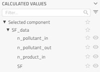
SF_data: Stoichiometric factor for the feed (SO2 and HCl) is calculated from the plant data. Stoichiometric factor is defined as moles of fresh sorbent added to the feed/moles of pollutants (SO2 and HCl) removed from the feed. (Note that SF is unitless.)
-
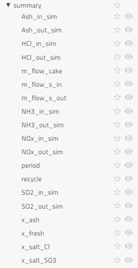
summary: Key variables of interest are outputted in the summary table for ease of reference
Simulation and Results🔗
To run the model (FlueGasTreatment.Tests.BagFilter_LW_SO2HCl), click on the play button in the canvas.
-
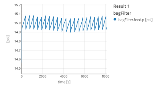
Once the simulation has run successfully, drag and drop the variables of interest in the canvas to obtain their time trajectories. Click on the eye icon (sticky) next to these variables and drag the slider at the bottom of the canvas to display their values at different points in time.
-
Summary section in the results (calculated values) contains some key output variables of the simulation.
-
The tutorial plots a few key variables of interest from the summary section and SF (stoichiometric factor) from the components: SF_sim and SF_data.
-
From the variables in the summary section, drag and drop SO2_in_sim and SO2_out_sim in the canvas (one by one) and plot them in the same graph.
-
Repeat the above for HCl_in_sim and HCl_out_sim; Ash_in_sim and Ash_out_sim. Now click on SF_sim in the canvas and plot SF. In the same graph, plot SF from SF_data.
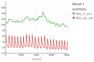
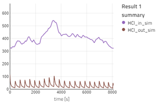
- If you visualize the graph of SO2_in_sim and SO2_out_sim, you will notice the outlet concentration of SO2 is quite less than the inlet concentration, as expected. The observation is similar for HCl. The outlet concentration for SO2 and HCl is fluctuating a lot: the concentration decreases and then suddenly spikes high and then it decreases again. This is because when the fresh sorbent reacts with the pollutants, the concentration of the pollutant decreases. The spike occurs during the time we remove the reacted sorbent from the bag filter. For more information, you can read the information section for the bag filter.
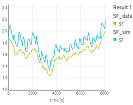
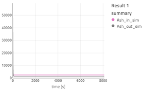
- The concentration of ash also decreases after entering the ESP. SF (stoichiometry factor) from the simulation result and the plant data are very close. You can also plot more variables if you desire.
Congratulations, you have learned how to use the catalytic bag filter model to treat flue gas emissions!