Clean Aircraft
Outline🔗
- Introduction
- What are we building?
- What will you learn?
- Performance Overview
- Weight vs Range simulation
- Mass Estimation
- Electrification
- Booster Power Table
- Aircraft Dynamics Library
- Integration
- Comparison Hybrid Electric vs Conventional
- Conclusion
- References
Introduction🔗
Current challenge in the aerospace industry is to develop technologies enabling cleaner aviation. Clean aircraft concepts go from fully electrified, hybrid-electric (series or parallel) to alternative fuels such as Sustainable Aviation Fuels (SAF) or Hydrogen.
Before Start: You will need approximately 1 hour to complete this tutorial
You will need the libraries:
- Aircraft Dynamics Library (ADL)
- Electrification Library (EL)
- Modelon Base Library (MBL)
What questions are we answering?🔗
When exploring clean aircraft, the key questions center around getting the same kind of range as conventional fuels. Clean aircraft introduces new unknowns such as weight and performance. This tutorial describes the workflow to build model, experiments and results in order to explore the relationship between electrification of an aircraft, fuel consumption and range.
What are we building?🔗
In this tutorial an electrified aircraft model will be built with basic assumptions on the electrical system and shaft power intake – using off the shelf models from Modelon Impact libraries (Aircraft Dynamics, Jet Propulsion and Electrification).
Comparisons will be made against the conventional propulsion system to explore the compromises that need to be made to reduce fuel consumption while increasing range of the aircraft. The resulting model will have the backbone that establishes the foundation upon which the user can build more complex systems to represent hybrid propulsion technology.
What will you learn?🔗
- re-use of an existing model
- integration of different libraries
- implementation of user assumptions into existing models
Performance Overview🔗
In this tutorial, aircraft performance is divided into 7 categories:
- Takeoff and landing
- Climb
- Range
- Speed
- Maneuverability
- Stability
- Fuel savings
The focus of this tutorial will be on the Range and Fuel economy of the aircraft, this can be analyzed through a Weight vs Range graph:
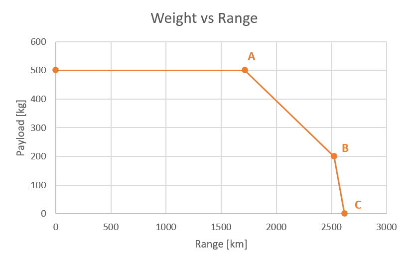
Point A is at the Maximum Take off Weight (MTOW), which is the maximum weight that the aircraft can carry due to physical constraints of the design and type of aircraft. At point B, the design “sacrifices” cargo mass to fill in our fuel tanks. However, it is only possible to fill in the tanks up to certain value limited by the capacity of the tanks itself. After this we can only add range by dropping cargo mass, which brings to point C.
The slope between point A and B is the fuel efficiency of our aircraft, this means that the additional fuel in the tanks will take us approximately 807 km further in range.
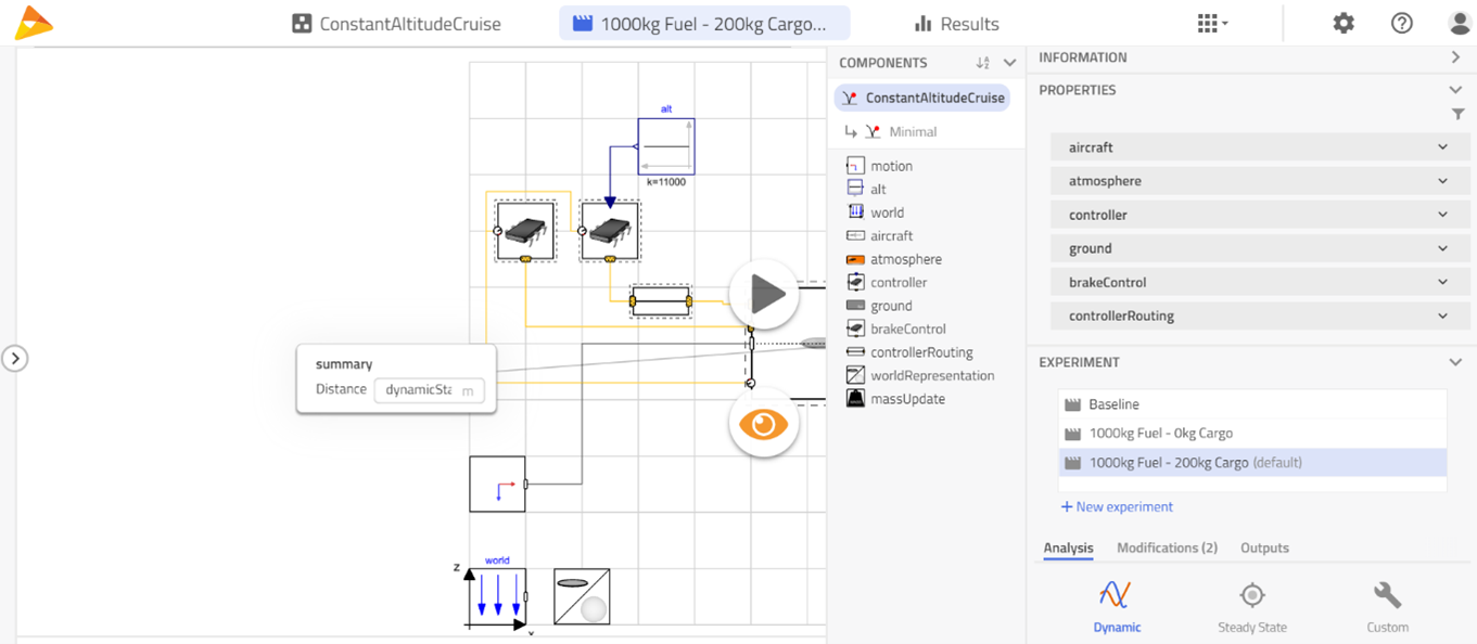
Weight vs Range Simulation🔗
- Duplicate to the workspace the example from
AircraftDynamics.Examples.ConstantAltitudeCruise. - In the Experiment mode, change the stop time to 50000s.
The example set up is defined to stop the simulation at the time the fuel runs out, this feature makes it perfect for the tutorial focus on weight vs range. The main assumptions of this Test Rig are :
- Based on BizJet architecture, 2 Degrees Of Freedom (DOF)
- Constant Altitude
- Constant Angle of Attack (at L/D max)
- Changing fuel mass, the model will run until all fuel is burned
- Fuselage Weight = 2522 kg
Aircraft architecture plays an important role on the weight vs range behavior but the focus of this tutorial is on the system level interactions, booster power, fuel consumption and electrical system, hence the same scope can be applied to a different Aircraft architecture like a B737.
Mass Estimation🔗
For the purpose of this tutorial, make further changes/assumptions to the masses.
- First assume the maximum weights of cargo and fuel
- 500 kg, Maximum Cargo weight ~ 20% of Fuselage weight
- 1000 kg, Maximum Fuel weight ~ 40% of Fuselage weight
- Then, for the Maximum Take Off Weight (MTOW) assume this limit to be at 3722 kg. Normally the aircraft owner would like to take the maximum cargo weight (500 kg). But taking into account fuselage weight (2522 kg), we will only have 700 kg left for fuel (70% of Maximum Fuel Weight).
- MTOW = 3722 kg = Fuselage + Maximum Cargo + 70% of Maximum Fuel Weight
- MTOW = 3722 kg = 2522+500+700
- Inspect the
aircraftcomponent, change thepower.fuel.m_fuel_startto 700 kg andaircraft.systems.mto 500 kg as follows:
-
This set up will be our baseline. Simulate the model.
-
On the Result tab, add a sticky for
aircraft.summary.Distanceand check the end of simulation time with the scroll to see the Maximum distance achieved with the Baseline setup.
- Create two experiment set up with 200 kg and 0 kg for cargo mass and 1000 kg fuel mass (for both).
- Next, get the Maximum distance for each of the experiments and build the following table, with which a plot of weight vs range can be obtained as well.
| Experiment | Input: cargo mass [kg] | Input : fuel mass [kg] | Result : range [km] |
|---|---|---|---|
| Experiment A | 500 | 700 | 1716.81 |
| Experiment B | 200 | 1000 | 2523.277 |
| Experiment C | 0 | 1000 | 2619.923 |
Electrification🔗
In this section we will edit the needed models from our Aircraft Dynamics Library in order to add the electric functionality. To organize the models properly, create the Workspace structure as below.
- Workspace
- Power
- Examples
- Engines
- EngineDeck
- FuelConsumption
- Electrical
- Examples
- Examples
- Power
Since we are going to modify connections and components we will need to duplicate some models, while others can be dealt with a extend procedure.
According to the following table, duplicate or extend the models from Aircraft Dynamics Library into the Workspace.
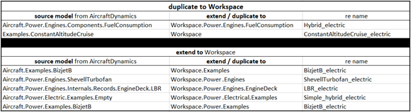
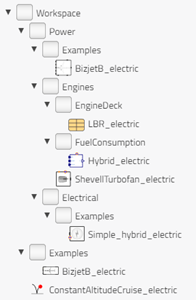
The workspace should look like the following figure.
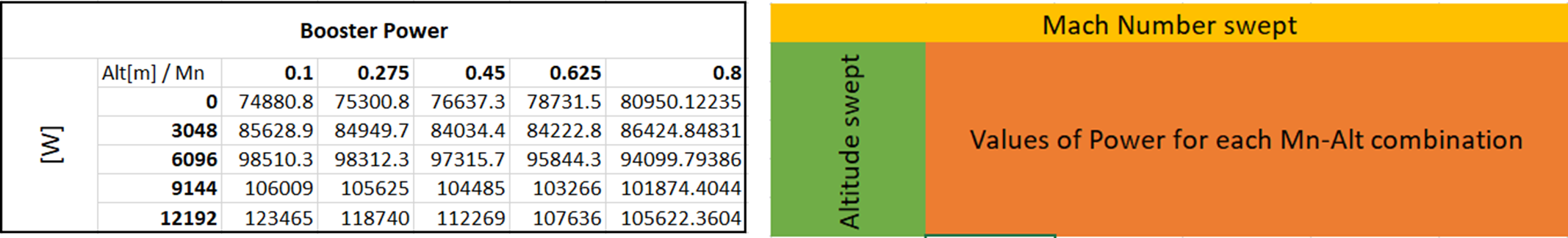
Booster Power Table🔗
To provide the aircraft model with the information about the booster power going into the engines, a table must be introduced.
Such table can be obtained by running a simulation from JetPropulsion.Experiments.GearedTurbofan.Cruise_offDesign with a sweep
of Mach number and Altitude (using range operator) and taking 20% of the power required by the core section of the fan,
this means; BoosterPwr = f(Mn, Alt).
For simplicity, the table is provided here:
parameter Real elecPwrIn_table[:,:] =
[ 0, 0.1, 0.275, 0.45, 0.625, 0.8;
0, 74880.832, 75300.822, 76637.286, 78731.542, 80950.122;
3048, 85628.852, 84949.745, 84034.439, 84222.779, 86424.848;
6096, 98510.296, 98312.285, 97315.691, 95844.330, 94099.794;
9144, 106008.650, 105624.619, 104484.759, 103266.176, 101874.404;
12192, 123464.803, 118739.560, 112269.200, 107635.914, 105622.360];
Tip
if you wish to input the data in ft or horse power you will need to include
.Modelon.Units.Conversions.from_ft and .Modelon.Units.Conversions.from_hp
at each of the elements on the table i.e.
.Modelon.Units.Conversions.from_hp(74880.832)
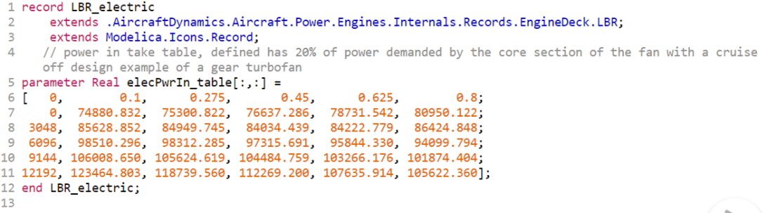
Note the modelica format of the table is as shown in the following figure.
Add the table elecPwrIn_table (copy-paste from above) to Workspace.Power.Engines.EngineDeck.LBR_electric, your new record should
look similar to the following figure.
Aircraft Dynamics Library🔗
Power Specific Fuel Consumption
Theory of shaft power off takes (as described in Reference 2) hold for the intake of power coming from the electrical system of the aircraft. Power intake will be reflected in the fuel flow and can be represented with delta Thrust Specific Fuel Consumption (SFC_Fn)
where, Fn is the net thrust, mass_flow_FP is the fuel flow savings due to the power intake and can also be represented as :
where, SFC_P is Power Specific Fuel Consumption [kg/(s*kW)]
At this point we can introduce the Shaft Power Factor kp :
And use kp to relate the fuel flow due to the power intake with the Thrust Specific Fuel Consumption
From equation (4) the Shaft Power Factor kp is kept constant at 0.00224 but ideally it will change with Mach Number and Altitude.
SFC_Fn are the tables available in ADL record LBR (tsfc_table), P is provided by the newly created booster Power table elecPwrIn_table.
Fuel Consumption Savings Modeling
To represent equation (4) we need to make some modifications to Workspace.Power.Engines.FuelConsumption.Hybrid_electric
- On the Sizing tab, change the
EngineDecktoLBR_electricas shown in the following figure.
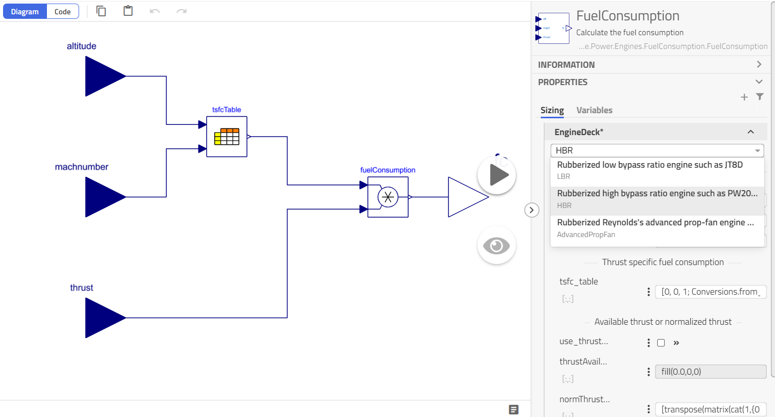
Warning
Double check you're adding the model from your Workspace.
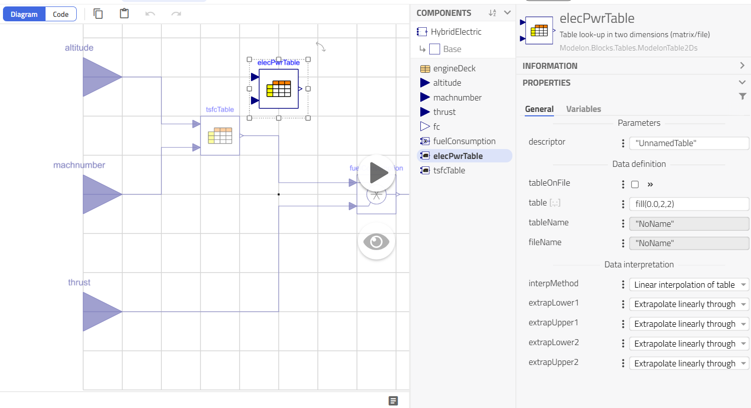
- Add a table block by drag and drop from
Modelon.Blocks.Tables.ModelonTable2Dsand set the value table = engineDeck.elecPwrIn_table, rename thisModelonTable2DsaselecPwrTable.
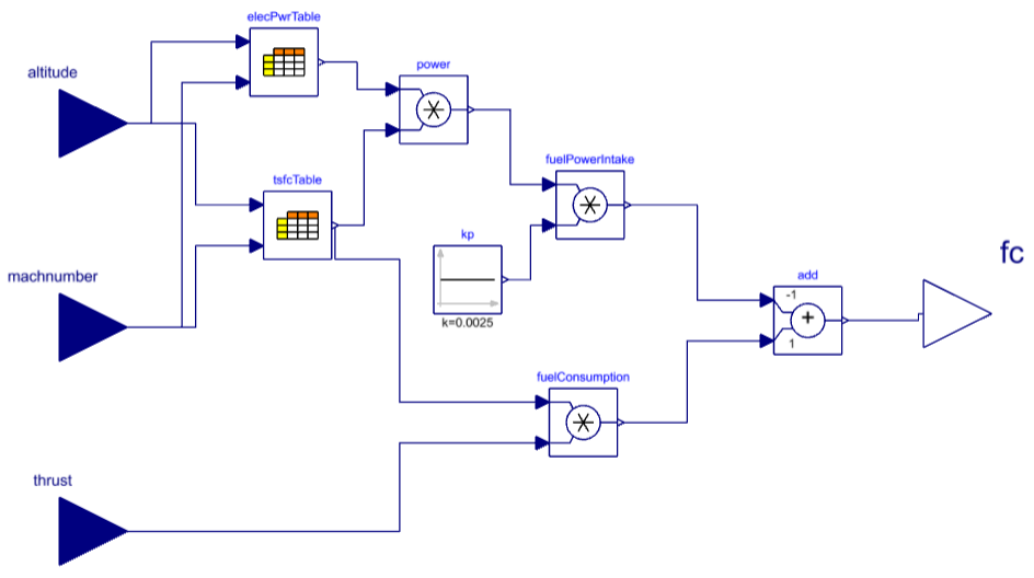
-
Add 2 product blocks from
Modelica.Blocks.Math.Productand rename them as power and fuelPowerIntake, then add a constant block fromModelica.Blocks.Sources.Constant, rename it as kp and set k =0.0025, finally add an addition block fromModelica.Blocks.Math.Addand set k1 = -1. -
Connect the blocks like shown in the following figure:
The power given by the elecPwrTable needs to be connected to our electrical network, we will need a signal power source to read the power
and convert this to electrical current, one DCplug to create the connection of the Fuel consumption model with other models in the engine
and one dcSplitter to separate positive and negative pin of the DCplug and connect the signal power.
- Drag and drop the models from the following paths.
- Signal power->
Modelon.Electrical.Analog.Sources.SignalPower - DCplug ->
Electrification.Electrical.Interfaces.DCPlug - dcSplitter ->
Electrification.Electrical.DCSplitter
- Finally, connect the electrical components as shown in the next figure.
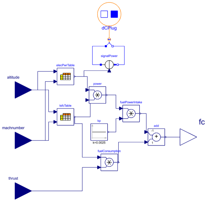
The Hybrid_electric model shows the modeling of the equation (4) and relates the fuel savings that we will obtain due to a power intake.
Engine with DC connection🔗
The new fuel consumption model Hybrid_electric created in the previous step needs to be added to our
Workspace.Power.Engines.ShevellTurbofan_electric model.
- On the parameter browser panel, under the General tab change the fuel consumption model. Select from the drop down menu our newly
created
Hybrid_electricmodel.
Warning
Double check you're adding the model from your Workspace.
-
Next, add a DCplug from
Electrification.Electrical.Interfaces.DCPlugand connect this to the fuel consumptionHybrid_electricmodel. -
The engine model should look similar to the next figure.
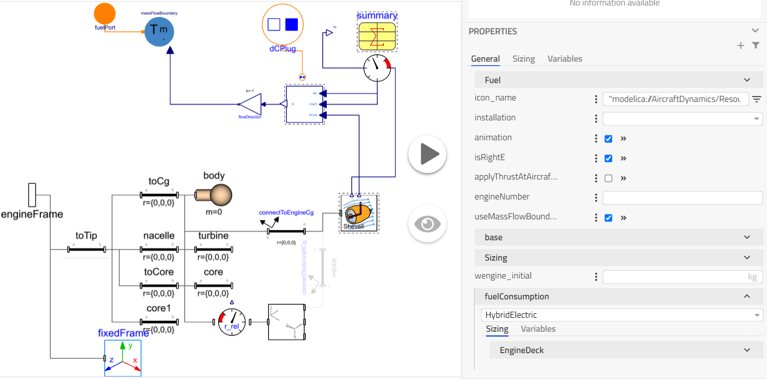
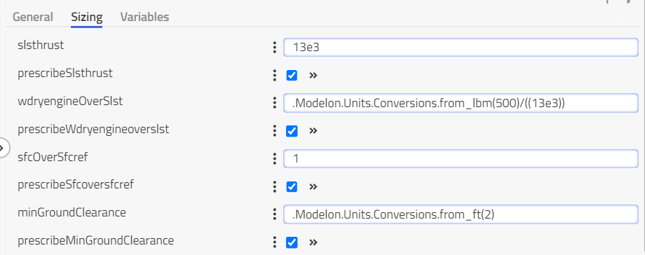
- In order to compare hybrid versus the conventional propulsion model (ConstantAltitudeCruise) we need to parameterize the
ShevellTurbofan_electricwith the same sizing, i.e. sea level thrust, clearance of the engines to the ground, reference ratio for SFC, etc. On the right hand side panel, at the Sizing tab set the following parameters:
slsthrust = 13e3wdryengineOverSlst = .Modelon.Units.Conversions.from_lbm(500)/(13e3)sfcOverSfcref = 1minGroundClearance = .Modelon.Units.Conversions.from_ft(2)
- Next, on the same sizing tab change the
EngineDeckto the newly createdLBR_electricand theRubGeotoLBR. Finally, select the body element and on the Mass and Inertia tab set m=0, since we are not considering the engine weight in this example.
Electrical Power🔗
We need to edit the electric distribution system Workspace.Electrical.Examples.Simple_hybrid_electric of the aircraft to include the electrification of the engines,
- Drag and drop a DCplug to connect the electric distribution system with the engines, a voltage source to provide the system the needed voltage for the power demanded and also a DCTripleSensor to watch on the power. The models can be found at,
- DCplug :
Electrification.Electrical.Interfaces.DCPlug - DCVoltage:
Electrification.Electrical.DCVoltage - DCTripleSensor :
Electrification.Electrical.DCTripleSensor
- Next, select the body model and at the Mass and Inertia tab change the mass of the electrical system m=100. The electric distribution system of the aircraft should look like the next figure.
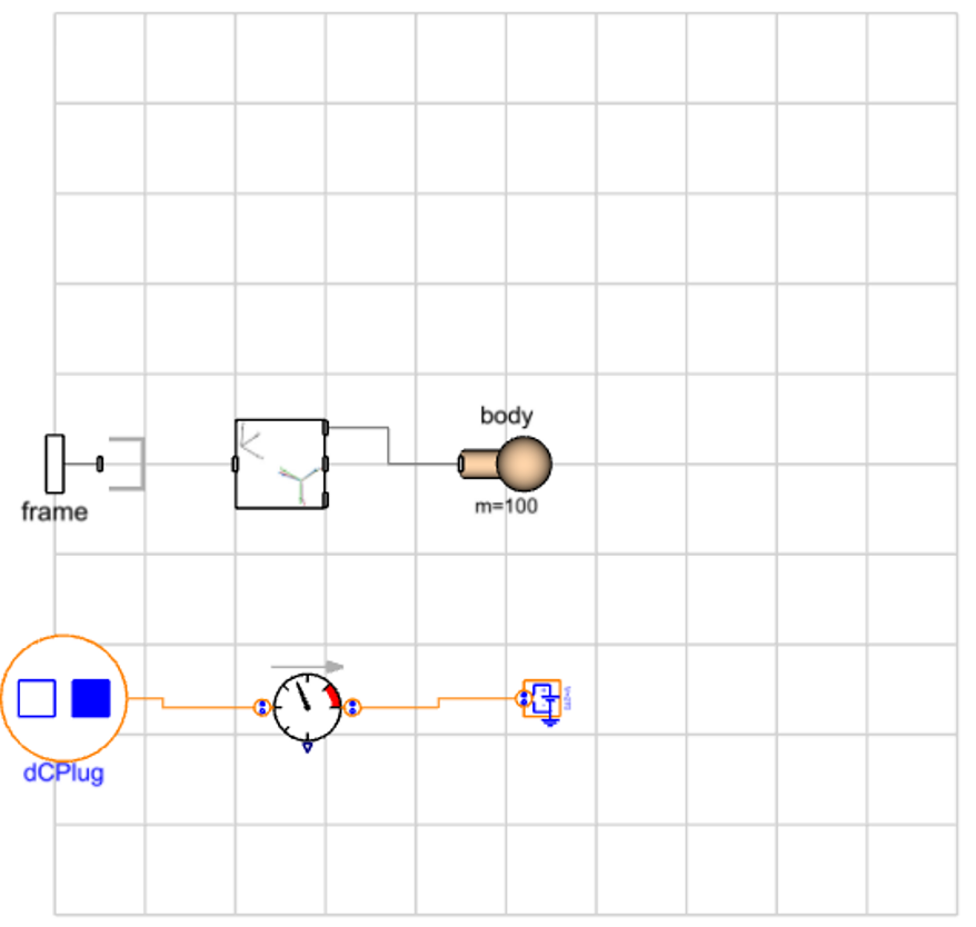
For the purpose of this tutorial we have not added any battery system in order to be able to compare with the conventional system at the most fundamental level.
Integration🔗
Power Model🔗
In the previous steps we have created the backbone elements to electrify our aircraft, now we need to implement and connect them.
- On the graphical interface of our power example
Workspace.Power.Examples.BizJetB_electricchange engine 5 and 6 toShevellTurbofan_electricand the electric element toSimple_hybrid_electric, connect the DC plugs from the engines to the electric element.
- Finally we need to parameterize the power model in order to compare with our conventional propulsion example ConstantAltitudeCruise, change the
fuelelement by selecting it and choosing from the drop down menuVariableMassmodel, inspect the fuel element and selecttoMassmodel, set the vector r to {17,0,-1.7}
Note
The toMass model sets spatial coordinates of the fuel tank, and will impact the flight dynamics.
Aircraft Model
- Next, at our aircraft example
Workspace.Examples.BizjetB_electricchange the power declaration to use our newly created power template
Workspace.Power.Examples.BizJetB_electric
The Aircraft model also needs to be parameterized in order to compare with our conventional propulsion example ConstantAltitudeCruise, the main assumption here is the angle of attack being constant at L/D Maximum with the Shevell aircraft coefficients.
- Inspect the model to
airframe.aeroand change the force definition toParabolic2. This will limit our aircraft movement to 2 degrees of freedom and set the coefficients as shown below.
- S = 19.51
- CDo = 0.026
- K = 0.045
- Next in the aero model change the sensing model to
PseudoAlphaand inspect it to change atdE2alphathe following variables,
- initType = Modelica.Blocks.Types.Init.InitialState
- y_start = (sqrt(0.026/0.045 + 0.0^2) - 0.0)/4.0 , values in the y_start formula are the coefficients used by our forces model
The following GIF shows this procedure.
Business Jet Electric model
On our Workspace.ConstantAltitudeCruise_electric select the aircraft model and on the drop down menu choose our newly created BizjetB_electric aircraft
model and change the simulation time to 50000s. We now have our electrified example of a business jet.
Comparison Hybrid Electric vs Conventional🔗
Execute ConstantAltitudeCruise_electric with the same process as shown in Weight vs Range Simulation section of this tutorial, but take into account that
now we have 100 kg of weight on our electrical system, therefore the variation of the fuel mass should reflect upon this in order to not exceed the MTOW.
You should come up with a table with similar values to the following:
| Experiment | Input: cargo mass [kg] | Input : fuel mass [kg] | Input : fuel mass hybrid [kg] | Result : range base [km] | Result : range hybrid [km] |
|---|---|---|---|---|---|
| Experiment A | 500 | 700 | 600 | 1716.810 | 1926.651 |
| Experiment B | 200 | 1000 | 900 | 2523.277 | 3025.640 |
| Experiment C | 0 | 1000 | 900 | 2619.923 | 3217.187 |
These points can be added to a Weight vs Range plot.
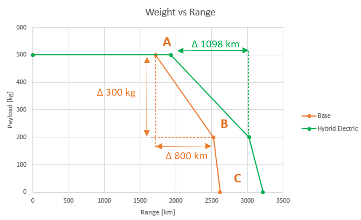
We can see that by including the 100 kg electric element providing unlimited power as required by the core fan section of our engines, the aircraft will be able to travel further. In this example 300 kg of fuel-payload trade off will give 800 km of range on our base model, while the Hybrid Electric model will give 1098 km with 300 kg.
Conclusion🔗
With the idealized assumptions made in this tutorial, it is clear the gain of including hybrid electric propulsion system. We save fuel and obtain range without sacrificing cargo/passengers. In real life we could expand the presented work in mainly three areas,
- Power Factor kp : This power factor could be better modeled in function of Altitude and Mach number that relates the characteristic of fuel consumption to the power intake from our electrical system. Such characteristics can be generated empirically and implemented in the form of tables and/or control model
- Electric System : The relation of power/mass of the electrical system can be further expanded to represent better real life examples
- Definition of Booster Power : This definition will be a function of the application of the aircraft and the electrical system itself
In spite of the assumptions presented in this tutorial, we have laid down the foundation and created a model (with drag and drop) that will work as a backbone for more complicated simulations/modeling.
This model can be found in the IndustryExamples library under the Aerospace section.
References🔗
-
Jack D. Mattingly, William H. Heiser, David T. Pratt: Aircraft Engine Design, Second edition, American Institute of Aeronautics and Astronautics, 2002.
-
Dieter Scholz, Ravinka Seresinhe, Ingo Staack, Craig Lawson: Fuel consumption due to shaft power off-takes from the engine, Workshop on Aircraft System Technology, Hamburg, Germany, 2013.