Outline

Introduction
Plant Introduction
- System layout
- System components
- Nominal data
System Modeling Steps
- Step 1: Create a package structure
- Step 2: Define the components according to supplier data
- Step 3: Create test bench models
- Step 4: Build the complete Brayton cycle power plant
Tips

Brayton Cycle🔗

Introduction🔗

This is a step-by-step tutorial to learn how to build transient models of complex thermodynamic systems in Modelon Impact. We will model a closed Brayton cycle mainly using components from the Vapor Cycle library but the instructions are generic and can be applied to successfully build any type of thermodynamic system. The tutorial will teach you how to break down the system modeling process into smaller steps to succeed in the overall task.

You will need approximately 120 minutes to finish all tutorial steps.

Library versions: Modelon 4.3, VaporCycle 2.11.

Modelon Impact version: Modelon Impact 2.9.x (Release 2023.2)

Plant information🔗

The system to be built is a Brayton cycle with supercritical CO2 (sCO2) as the working fluid. A Brayton cycle is a thermodynamic cycle that describes the operation of a gas turbine. It exists in different variants and we will focus on a simple & closed Brayton cycle, i.e. that recirculates the working fluid. There is no phase change for the working fluid, it stays in the supercritical region.

System layout🔗

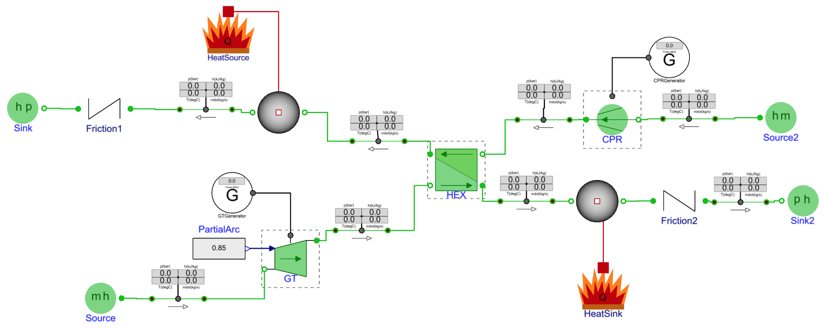
The plant to be modeled is a simplified version of the Vapor Cycle Library example found in VaporCycle.Experiments.RecompressionBraytonCycle.

Below, you’ll see the plant schematics and the Impact model including closed-loop controllers that you’ll be building step-by-step in the tutorial.

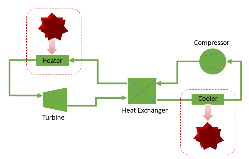
System components🔗

To model the main components shown in the plant layout, we’ll use the following models:

Gas Turbine:

VaporCycle.Expanders.TurbineStodola

Compressor:

VaporCycle.Compressors.DynamicCompressor

Heat Exchanger:

VaporCycle.HeatExchangers.TwoPhaseTwoPhase.CounterFlow

Heater/Cooler: (for ideal heat removal or addition)

VaporCycle.Tanks.Volume

Heat source/sink:

VaporCycle.Sources.HeatSource

The CO2 medium model valid in the supercritical region will be taken from

 VaporCycle.Media.Naturals.CarbonDioxideRef

We’ll also need the following auxiliary components:

Generator: (to visualize the power consumed/produced at a given frequency)

Modelon.ThermoFluid.Electrical.SimpleGenerator

Flow source:

 VaporCycle.Sources.TwoPhaseFlowSource

Flow sink:

 VaporCycle.Sources.TwoPhasePressureSource

Friction:Friction:

 VaporCycle.FlowResistances.GenericFlowResistance

Controller:

  Modelon.Blocks.Control.LimPID

Real input:

  Modelica.Blocks.Sources.RealExpression

Ramp:

  Modelica.Blocks.Sources.Ramp

Sensor:

  VaporCycle.Sensors.MultiDisplaySensor

Visualization:

  VaporCycle.Sensors.MultiDisplayVis_phTmdot

Legend description:

  VaporCycle.Utilities.Visualizers.

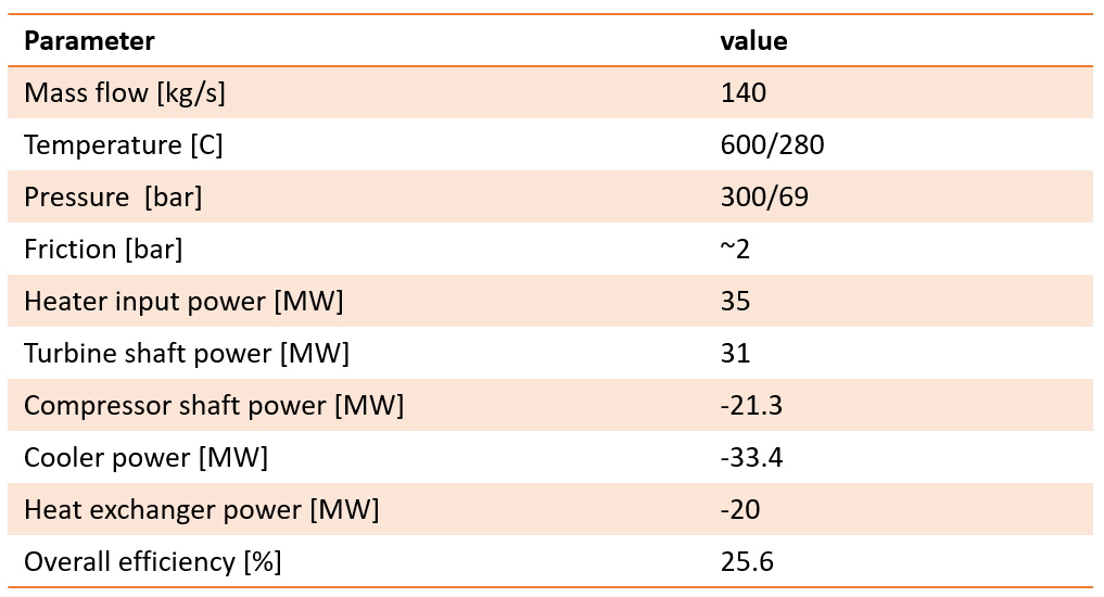
Nominal data🔗

Below, you’ll find the nominal data for flow, pressures and temperatures in the cycle.

System modeling steps🔗

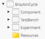
Step 1: Create a package structure🔗

A package structure needs to be created to store all models & experiments. Create a package

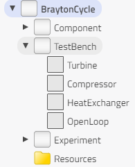
Let’s call the top-package BraytonCycle and create three sub-packages therein:

Component
TestBench
Experiment

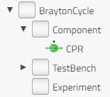
Step 2: Component parameterization using available data🔗

The Component package is meant to contain parameterized library models representing specific supplier components. Once they have been parameterized and eventually named according to some supplier catalog, they will be used as is in the system model or the test benches.

In this tutorial, we will assume that only the compressor is defined by supplier data. Let’s then add a compressor model in the Component package by extending VaporCycle.Compressors.DynamicCompressor from the Vapor Cycle Library:

The components have been renamed as follows for ease of understanding.

When assembling the complete system model, the gas turbine and the compressor component models will be taken from the Component package whereas the other components (heat exchanger, volumes, …) will be taken directly from the library. The parameters of the heat exchanger could eventually be adjusted in the test bench or directly in the system model to meet some requirements.

Parameterize the models inside the Component package🔗

Now we can parameterize, the compressor model inside the Component package. Simple compressor maps are used here to generate the targeted mass flow rate and efficiency. The values will be interpolated and extrapolated with table data.

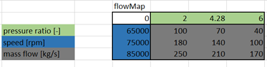
Go to “CharMap”, and add the maps as follows:

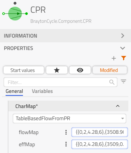
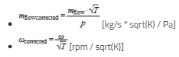
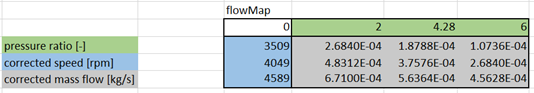
Compressor flow map: corrected speed and corrected mass flow rate are used flowMap = { {0,2,4.28,6},{3508.902626,0.0002684,0.00018788,0.00010736},{4048.733799,0.00048312,0.00037576,0.0002684},{4588.564972,0.000671,0.00056364,0.00045628} }
Before correction: the speed unit used in the map is rpm, while the generator speed unit is rad/s

After non-normalized correction

Compressor efficiency map: corrected speed and isentropic efficiency are used effMap = { {0,2,4.28,6},{3509,0.77,0.78,0.76},{4049,0.77,0.78,0.76},{4589,0.77,0.78,0.76} }

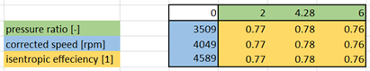
In this approach, the characteristics maps of the extended compressor will be a “fixed” parameterization, and they are valid if interpolation and extrapolation are reasonable. So the compressor with predefined and reasonable maps can be used without further modifications if not in extreme working conditions.

Step 3: Create test bench models🔗

Before assembling the complete system model, subsets of the plant will be isolated and simulated using boundary conditions defined by the nominal data. Test benches can be set up for various purposes:

To verify the parameterization of the models from the Component package in single-component experiments. This can be done both at the nominal point but also using time-varying boundary conditions. Refer to Compressor Test Bench.
To “design” the components (ex: heat exchanger) in a single-component experiment. The simulation is here mainly meant to find the right parameterization (ex: efficiency or geometry data) that achieves the desired performance (ex: duty, temperature) at the nominal point. Ideally, one could use a systematic approach to find the best parameters, using parameter sweeps or inverse steady-state simulation. Refer to Heat Exchanger Test Bench, SteadyState experiment and Multi-execution experiment.
To test the behavior of subsystems by assembling components that have already been tested. In the case of a closed thermodynamic cycle, it is typically a good idea to break the loop and not recirculate the working fluid. Closing the loop is done once the outlet values are aligned with expectations. Similarly, controllers can be introduced at a later stage to operate the model at various operating points. Refer to OpenLoop Test Bench.

We will set up four test bench models, i.e. one for each main component (turbine, compressor, heat exchanger) and one for an open loop system model. Open in the sense that it does not have any controller and the working fluid is not recirculated.

General steps to create a test bench

Decide the specific component to be tested
Add components to the canvas
Optional: Rename components at your convenience
Connect components
Optional: enable the main component to be replaceable. Useful if a given component is available with different parameterizations to reflect a catalog list.
Parameterize according to the nominal point data
Choose the solver and set up the experiment
Check simulation results
Change boundary conditions in a dynamic way to test the component behavior away from the nominal point

Connection rules🔗

The fluid connectors in all Modelon libraries exist in 2 versions (filled and hollow) and they are used according to some conventions that help the end user build complex systems robustly.

Filled (or Flow) connector is used whenever the component is computing and setting the mass flow rate at the port. A mass flow source would typically have a filled connector. Other components such as pressure loss models will also compute and set the flow at their ports based on the surrounding pressures.
Hollow (or Volume) connector is used whenever the component is setting the pressure at the port. This is valid for a pressure source but also for any “large” volume/storage that will compute the pressure from a mass balance across the component boundary.

It is recommended to always alternate filled and hollow connectors to avoid numerical issues when building a system model. If this is not possible, additional pressure loss models or volumes can be inserted between the components with similar connectors.

Refer to slides 20-24 in the Composing System Models training material.

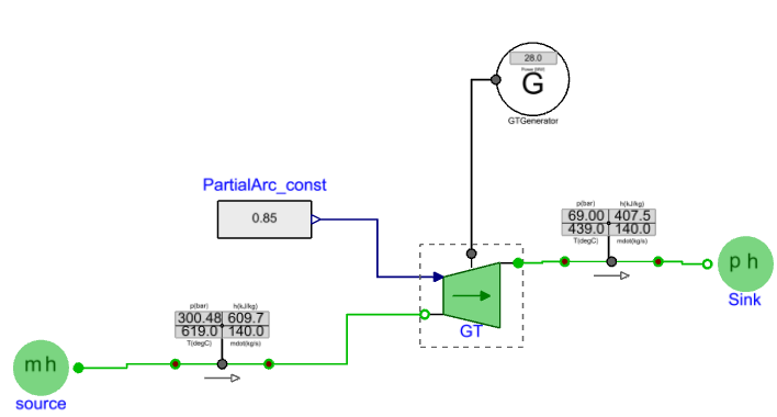
Turbine🔗

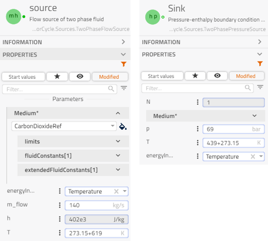
The working fluid s-CO2 with a mass flow of ~140kg/s and temperature of ~600C is expanded from 300 bar to 65 bar by the gas turbine.

Add Components to the canvas🔗

Turbine:

BraytonCycle.Component.Turbine.GT

Generator:

Modelon.ThermoFluid.Electrical.SimpleGenerator

Boundary source:

VaporCycle.Sources.TwoPhaseFlowSource

Boundary sink:

VaporCycle.Sources.TwoPhasePressureSource

Real input:

Modelica.Blocks.Sources.RealExpression

Multi-sensor:

VaporCycle.Sensors.MultiDisplaySensor

Visualization:

BraytonCycle.Component.Others.VisDisplay

Rename components🔗

Turbine: GT
Boundary source/sink: Source/Sink
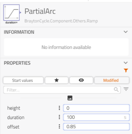
Real input: PartialArc_const
Generator: GTGenerator

Connect components🔗

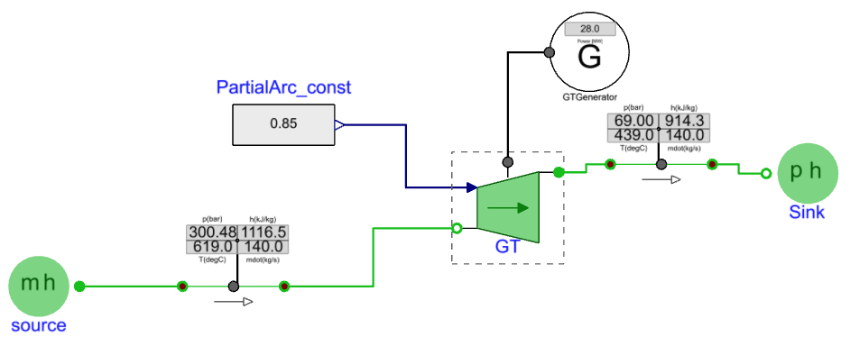
Observe that a hollow connector is always connected to a filled connector. The hollow connector at the turbine inlet indicates that pressure is set by some internal volume in the turbine. The initial pressure and temperature are also expected to be specified by the end user (see the Initialization tab below).

Parameterization🔗

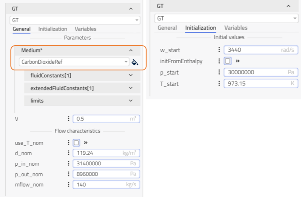
Gas turbine: GT🔗

Choose medium CarbonDioxideRef as the working fluid, and the path is:
```
VaporCycle.Media.Naturals.CarbonDioxideRef
```
Propagate the medium

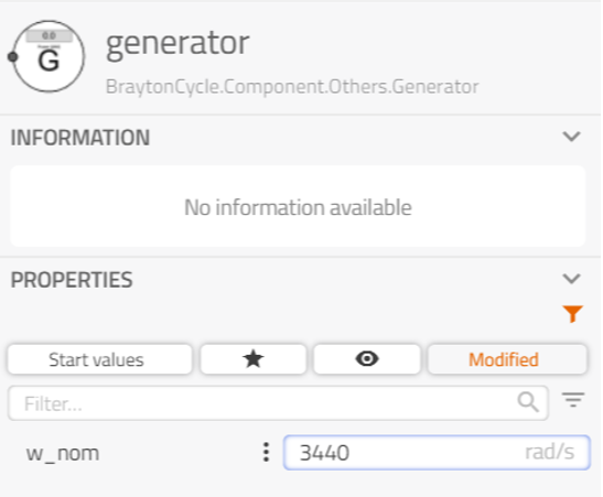
Generator🔗

The generator speed decides the turbine speed since the flanges are connected.

PartialArc🔗

The flow rate entering the turbine can be reduced by partial arc admission. The partialArc input needs to be specified to use the turbine model. Reasonable values range from 0.75 to 1. We’ll choose a constant value of 0.85.

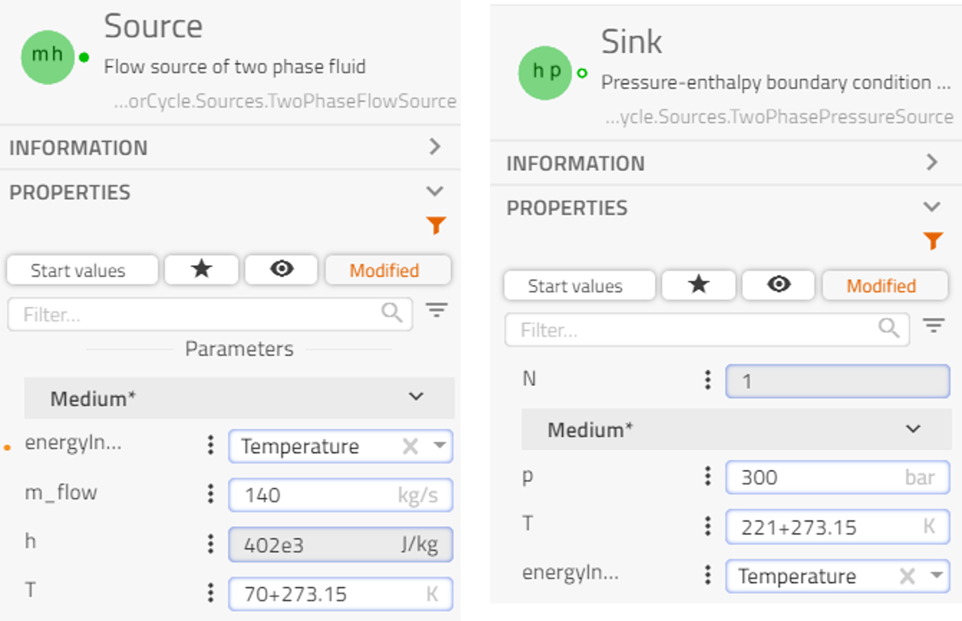
Source and Sink🔗

Set up the boundary conditions of mass flow rate, temperature and pressure.

Solver and experiment🔗

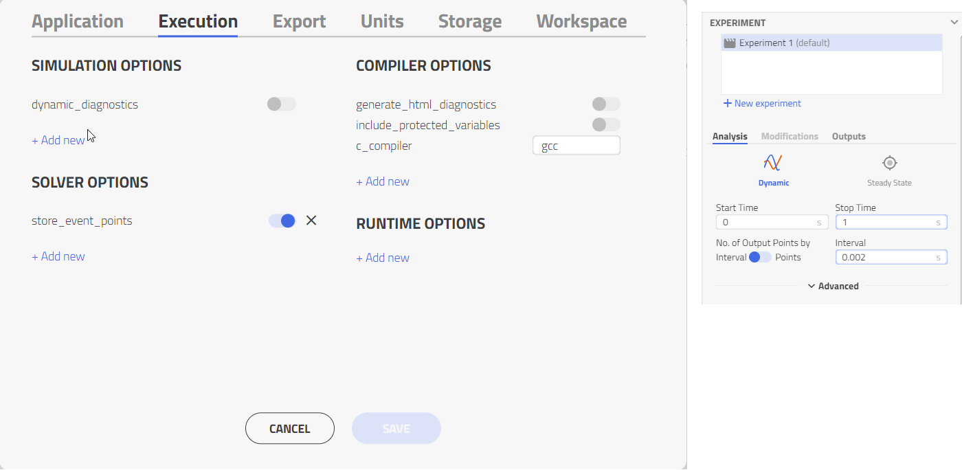
Simulation results🔗

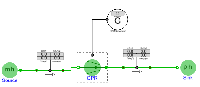
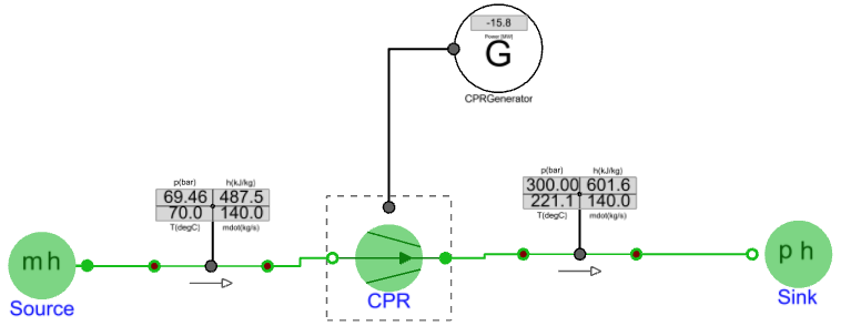
Compressor🔗

The compressor pressurizes the gas from 69 bar to 300 bar.

Add Components to the canvas🔗

Compressor:

    BraytonCycle.Component.Compressor.CPR

Generator:

    Modelon.ThermoFluid.Electrical.SimpleGeneratoraytonCycle.Component.Others.Generator

Boundary source:

    VaporCycle.Sources.TwoPhaseFlowSource

Boundary sink:

    VaporCycle.Sources.TwoPhasePressureSource

Multi-sensor:

    VaporCycle.Sensors.MultiDisplaySensor

Visualization:

    BraytonCycle.Component.Others.VisDisplay

Rename components🔗

Compressor: CPR
Boundary source/sink: Source/Sink
Generator: CPRGenerator

Connect components🔗

Observe that the connection rule is also respected here.

Parameterization🔗

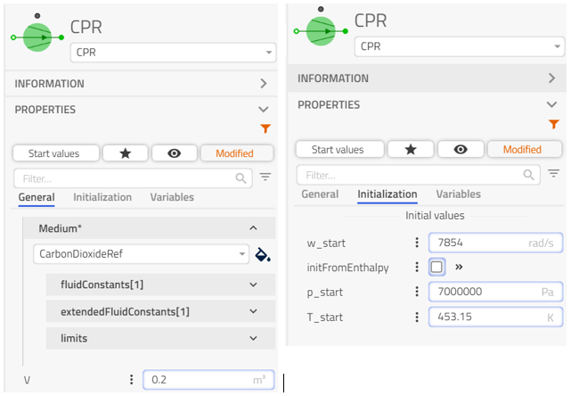
Compressor: CPR🔗

Choose medium CarbonDioxideRef as the working fluid, and the path is:

VaporCycle.Media.Naturals.CarbonDioxideRef.

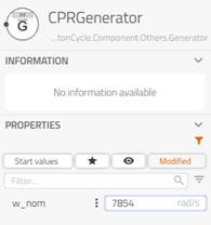
Generator: CPRGenerator🔗

The generator here is similar to the one used in the turbine test bench; its speed decides the compressor speed since the flanges of the shaft are connected

Source and Sink🔗

Set up the boundary conditions of mass flow rate, temperature and pressure.

Solver and experiment:🔗

Same setup as in Turbine Simulation results

Simulation results🔗

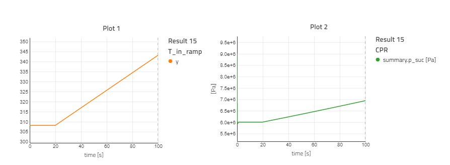
Dynamic response to increasing liquid temperature (T_in)🔗

Check the option “use_Th_in” in the “Source”
Add a ramp into the canvas: BraytonCycle.Component.Others.Ramp
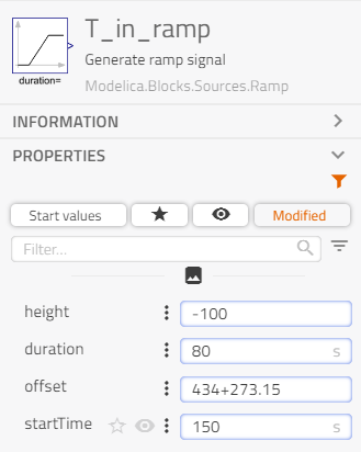
Rename “Ramp” to T_in_ramp

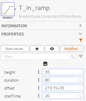
Parameterization of T_in_ramp

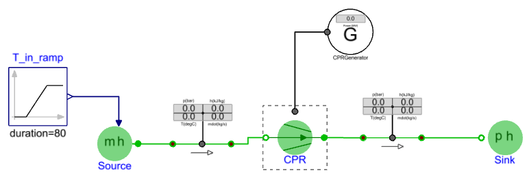
Connect the T_in_Ramp to the source
Dynamic results: the increasing temperature (Plot 1) of fluid entering CPR results in higher feed pressure (Plot 2).

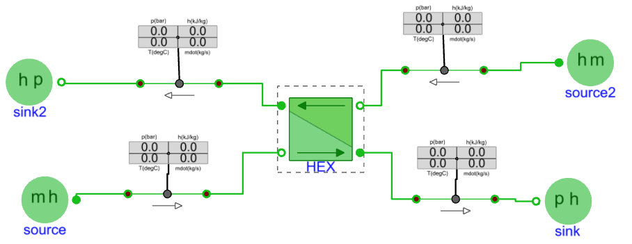
Heat Exchanger🔗

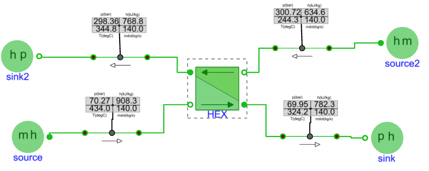
The heat exchanger preheats the gas streams exiting the compressor by the gas stream exiting the gas turbine from 244 degC to 411 degC.

Add Components to the canvas🔗

Heat exchanger:

VaporCycle.HeatExchangers.TwoPhaseTwoPhase.CounterFlow

Boundary source:

VaporCycle.Sources.TwoPhaseFlowSource

Boundary sink:

VaporCycle.Sources.TwoPhasePressureSource

Multi-sensor:

VaporCycle.Sensors.MultiDisplaySensor

Visualization:

BraytonCycle.Component.Others.VisDisplay

Rename components🔗

Heat exchanger: HEX
Boundary source/sink: Source/Sink/Source2/Sink2

Connect components🔗

Parameterization🔗

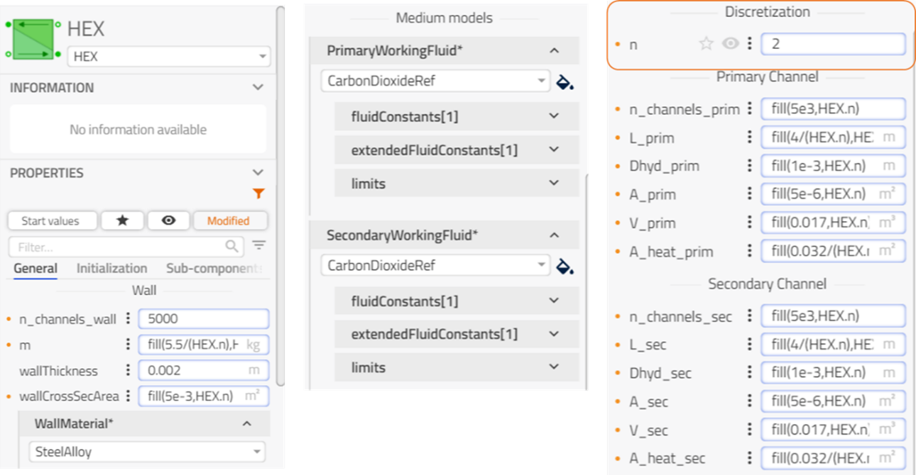
Heat exchanger: HEX🔗

Choose and propagate the medium CarbonDioxideRef as “PrimaryWorlingFluid” and “SecondaryWorkingFluid”
In “Discretization”, large “n” values lead to higher accuracy at the expense of a longer simulation time.
General setup

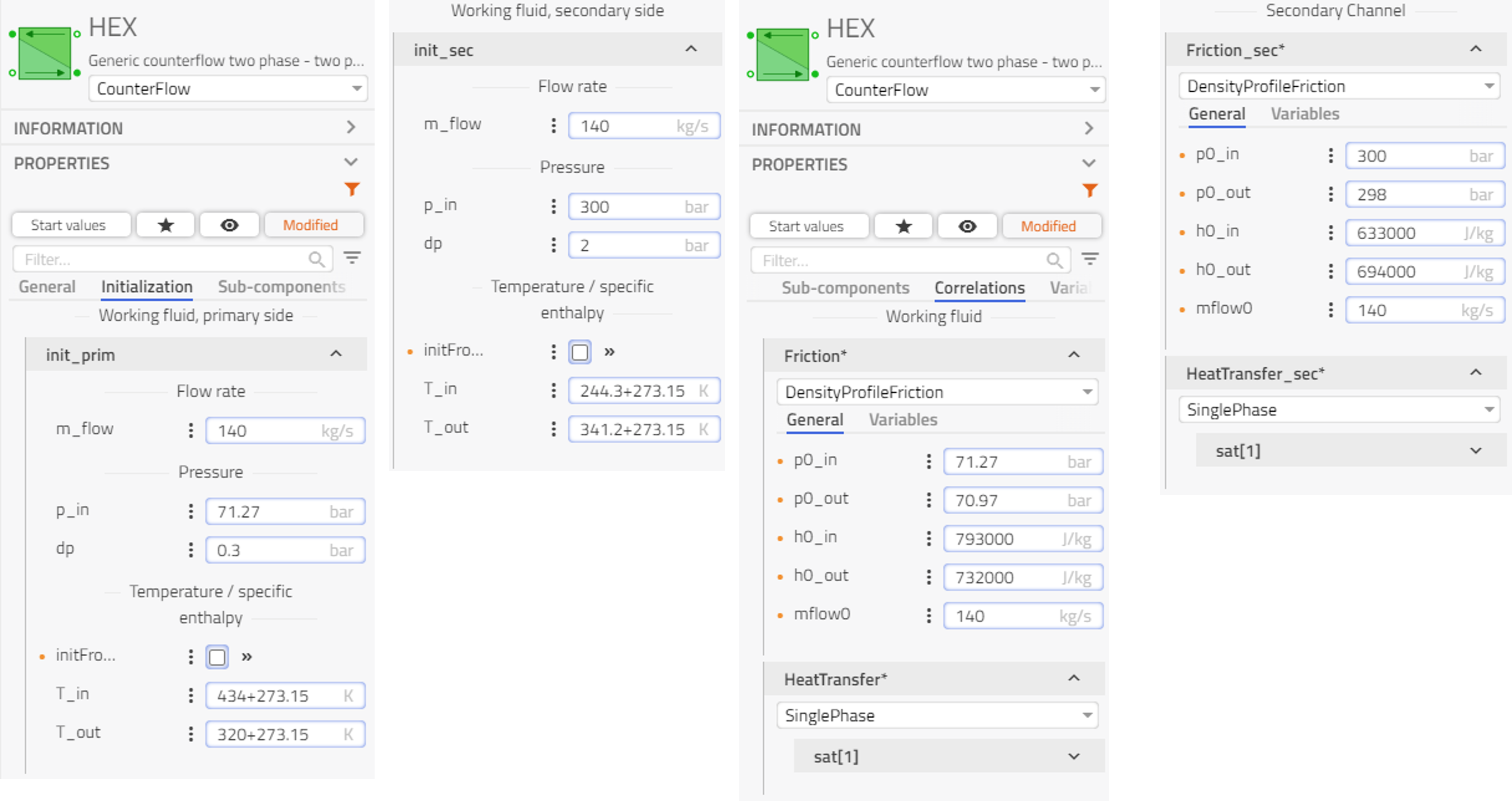
Initialization & Correlations.

Note

The heat exchanger model is a dynamic model and there is a need to specify its initial state in terms of temperature and pressure profiles for each side.

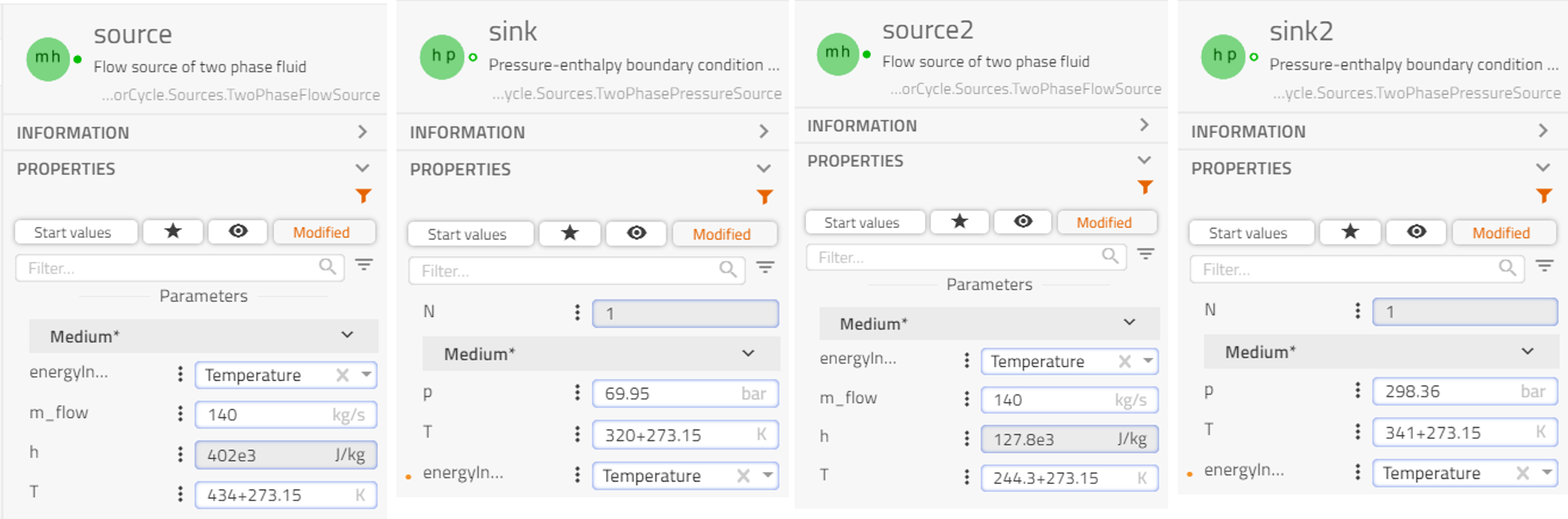
Source and Sink🔗

Solver and experiment:🔗

Same setup as in Turbine Simulation results

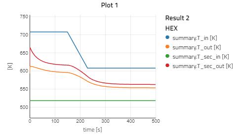
Simulation results🔗

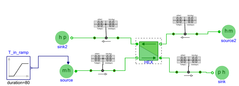
Dynamic response to decreasing inlet enthalpy of primary fluid🔗

Check the option “use_Th_in” in the “source”
Add a ramp into the canvas: BraytonCycle.Component.Others.Ramp
Rename “Ramp” to “T_in_ramp”
Parameterization of “T_in_ramp” and connect it to “source”

After connection

Set experiment stop time = 500 s.
Dynamic results: Decreasing temperature input from 707.15 K to 607.15 K affects the temperatures of primary and secondary fluid exiting the heat exchanger.

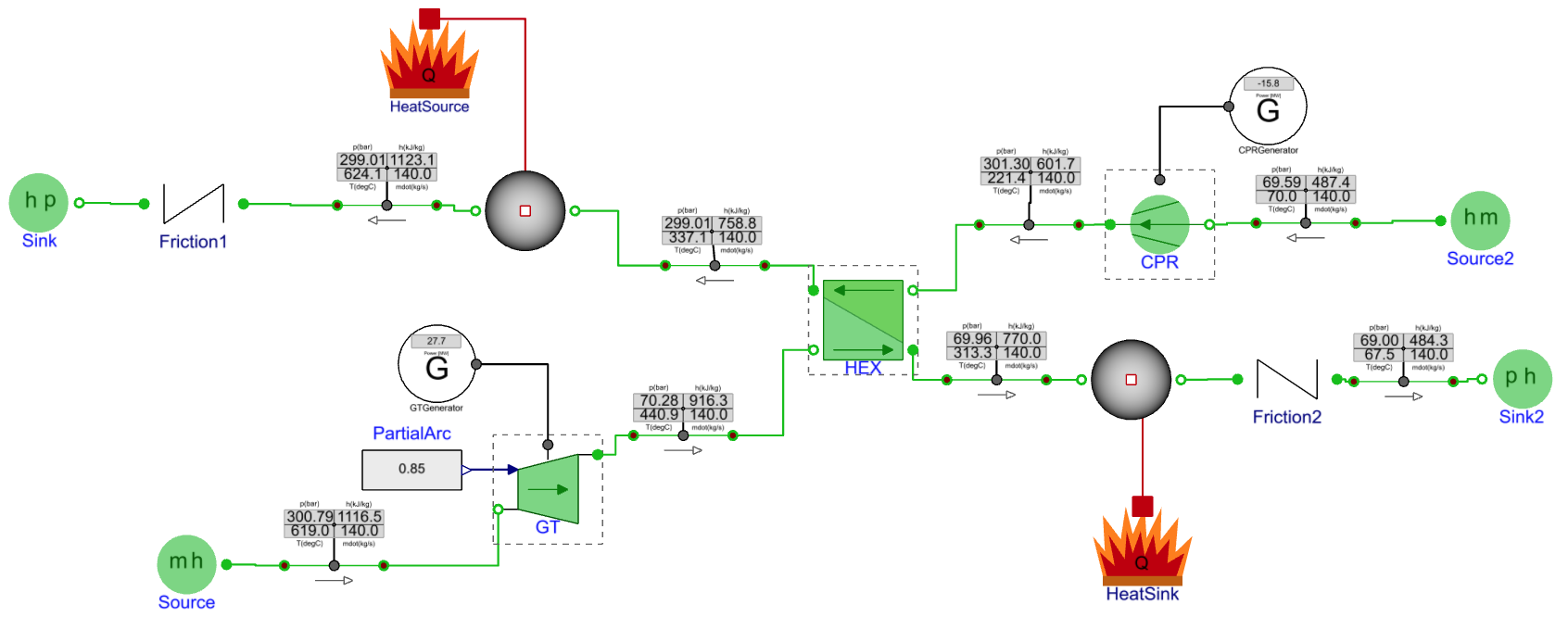
Open loop test🔗

This step aims at assembling most of the components that describe the full Brayton cycle but without recirculating the working fluid. Apart from the previously tested components (turbine, heat exchanger, compressor), a heater and cooler need to be added. The combination of an external heat source and a volume is used to describe an ideal heat addition or removal. At some point, this could also be replaced by heat exchanger models but this is not done in the tutorial. Simple friction models are also used to describe the pressure losses in the system, but also to avoid the numerical issues mentioned earlier.

Create an OpenLoop sub-package inside TestBench🔗

Copy the parameterized components from the TestBench models🔗

GT connected with GTGenerator from
```
    BraytonCycle.BenchTest.Turbine
```
GT connected with GTGenerator from
```
    BraytonCycle.BenchTest.Compressor
```

HEX from

    BraytonCycle.BenchTest.HeatExchanger

Add components to the canvas🔗

2 Volume:
```
 VaporCycle.Tanks.Volume
```
2 HeatSource:
```
 VaporCycle.Sources.HeatSource
```

2 Friction:

 VaporCycle.FlowResistances.GenericFlowResistance

Multiple sensor:
```
 VaporCycle.Sensors.MultiDisplaySensor
```

Multiple visualizer:

 VaporCycle.Sensors.MultiDisplayVis_phTmdot

Rename components🔗

Heater/Cooler
HeatSouce/HeatSink
Friction1/Friction2

Connect components🔗

Parameterization🔗

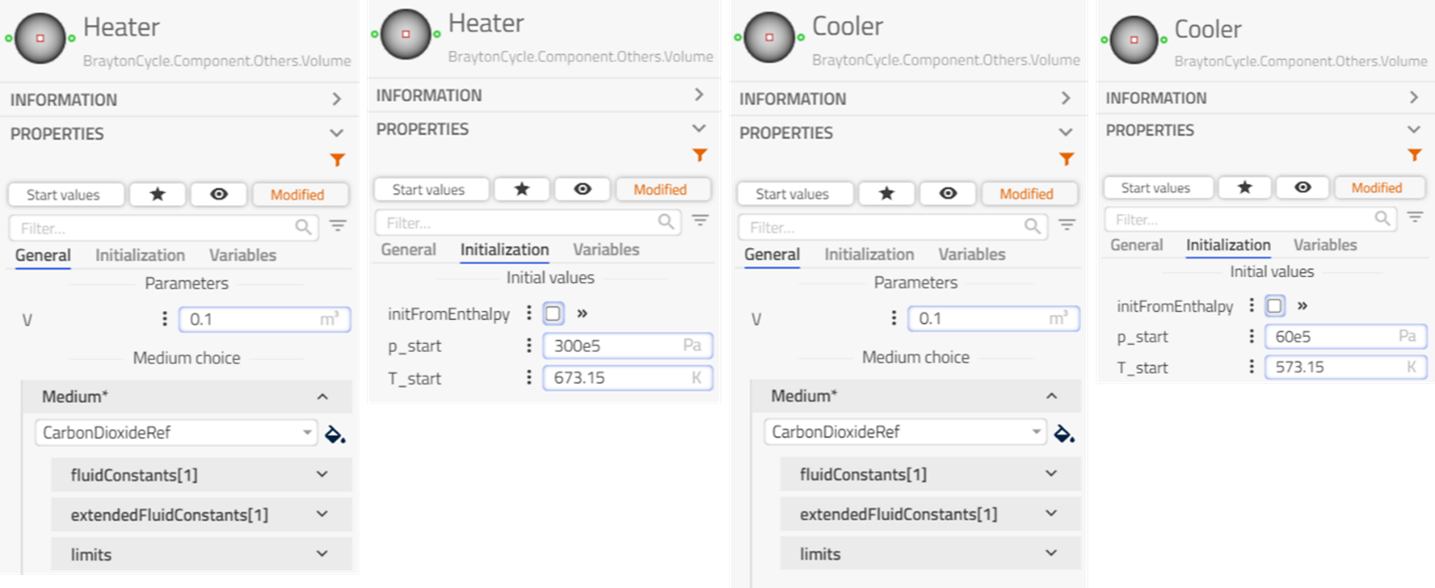
Heater and Cooler🔗

Volume model with heat source is used as heater and cooler, depending on the heat is provided or extracted.
Volumes:

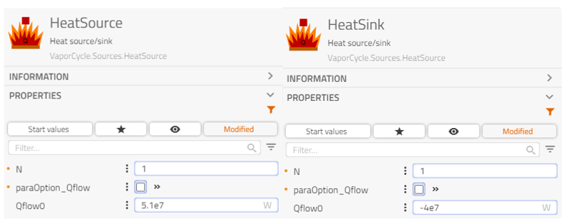
HeatSource and HeatSink: Negative value of Q_flow means extracting the heat, and positive means providing the heat. openloopheatsource

Solver and experiment:🔗

Same setup as in Turbine Simulation results

Simulation results🔗

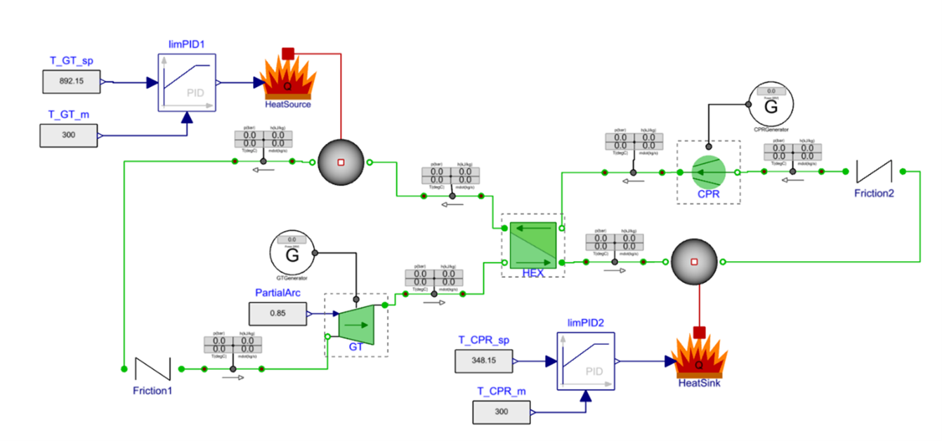
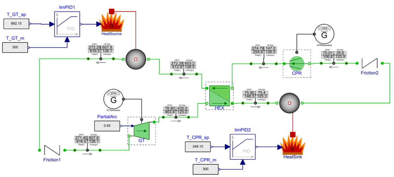
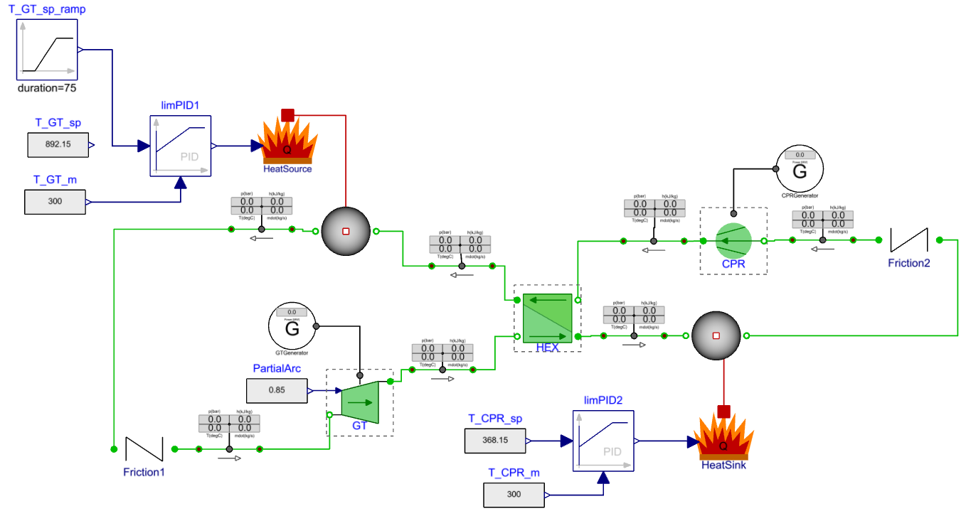
Step 4: Build the complete Brayton cycle power plant🔗

To have a complete Brayton cycle, the sources and sinks in the test bench OpenLoop are removed, the outlet of “Friction1” is connected to the inlet of “GT”, and the outlet of “Friction2” is connected to the inlet of “CPR”. Simple PI controllers have been added to control the heater/cooler and maintain the working fluid temperatures at their target values.

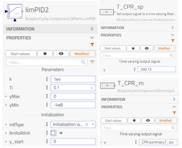
Add Components to the canvas🔗

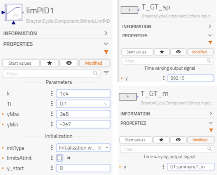
2 LimPID: Modelon.Blocks.Control.LimPID.
4 Real input: Modelica.Blocks.Sources.RealExpression

Rename components🔗

limPID1/limPID2
T_GT_sp/T_GT_m/T_CPR_sp/T_CPR_m

Connect components🔗

Remove the sources and sinks, connect the components, and close the loop.

Parameterization🔗

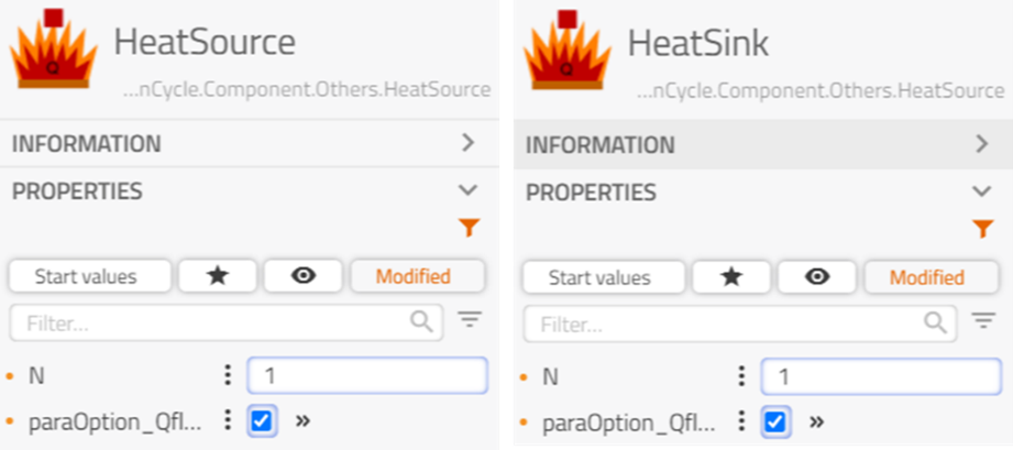
HeatSource and HeatSink:
- Check the “paraOption_Q_flow”, thus the Q_flow to the heat source can be manipulated by the PI controllers.

Controllers: the heat is controlled by PI controllers to maintain the temperatures of the fluid entering the compressor ”CPR” and turbine ”GT”, respectively.
LimPID1

LimPID2

Solver and experiment🔗

Same setup as in Turbine Simulation results

Simulation results🔗

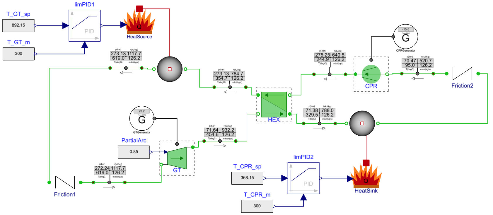
First assessment of the closed-loop response🔗

Verify that the temperature at the turbine and compressor inlet is well stabilized using the newly introduced controllers. Some deviations in the cycle mass flow rate and the pressure levels can however be found

the target mass flow rate is 140 kg/s, while the system mass flow rate is only ~126 kg/s.
the low-pressure side is around 69 bar and the high pressure is at 314 bar, while the system pressures define by the nominal data are 70 bar and 274 bar.

The compressor speed has a significant impact on the system mass flow rate and pressures and it can be adjusted for a better match. Increase the compressor nominal speed ”w_nom” in ”CPRGenerator” from 7854 rad/s to 9000 rad/s and re-simulate the system model.

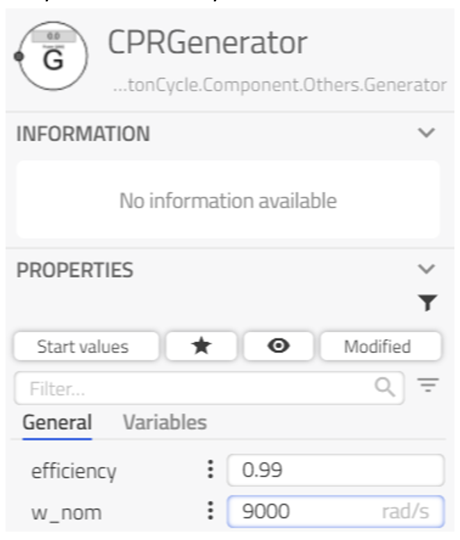
The mass flow rate is now more consistent with the nominal data but some deviation in the compressor outlet pressure can still be seen. The compressor map would need to be further adjusted for a better match.

Dynamic response to gas turbine inlet temperature change (T_GT_sp)🔗

Add the ramp to the canvas
```
 BraytonCycle.Component.Others.Ramp
```

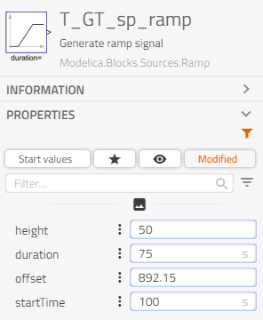
Rename it to: T_GT_sp_ramp
Disconnect T_GT_sp and connect T_GT_sp_ramp to limPID1

Set the stop time as 500 s
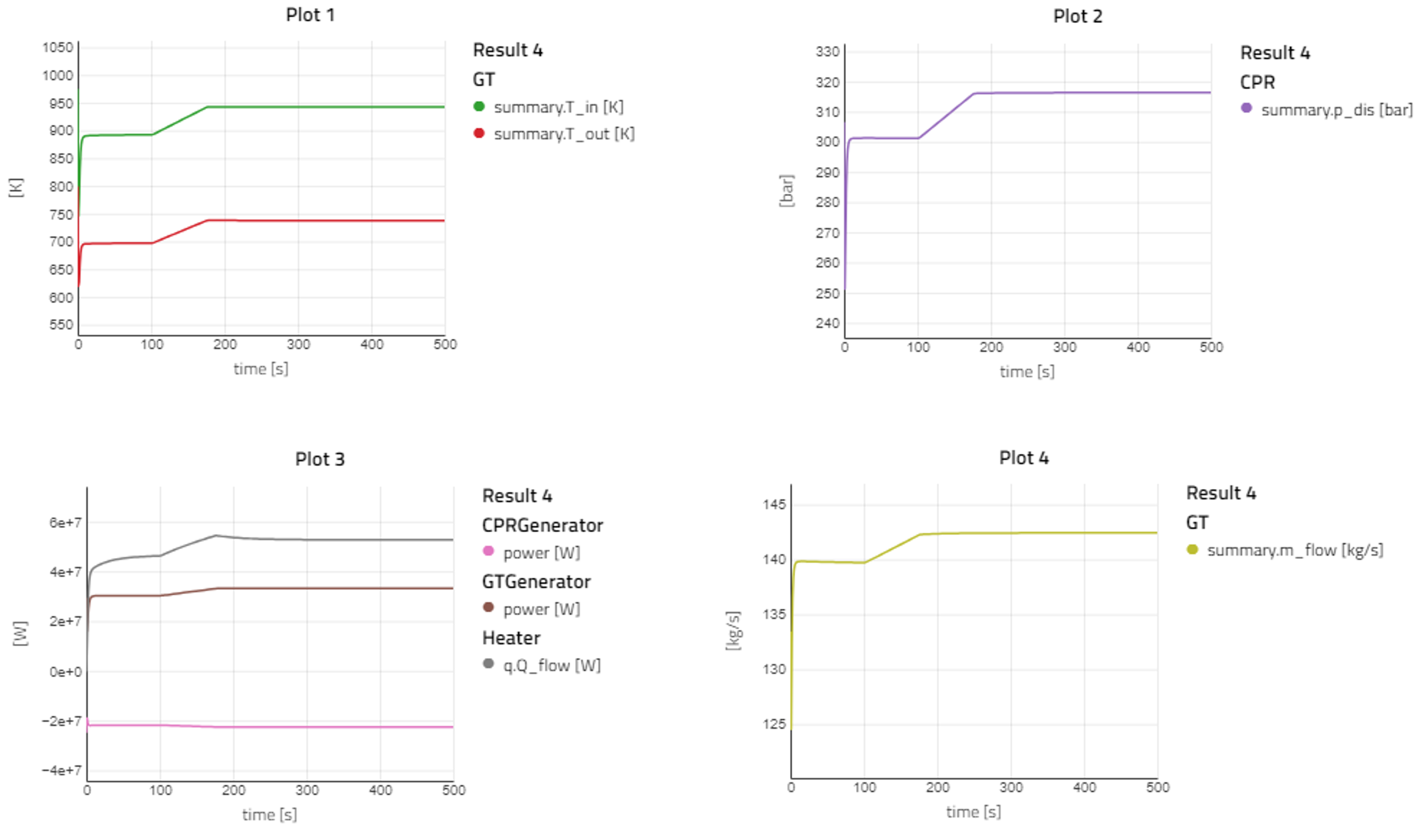
Dynamic results: increasing T_GT_sp (Plot 1: GT summary.T_in) results in
- increasing pressure of fluid exiting the compressor (Plot 2)
- higher power generated by the turbine and higher power consumed by the compressor (Plot 3)
- higher system mass flow rate (Plot 4)

Tips🔗

Replaceable component model for tests of different component variants
- Example: replaceable turbine

Edit it in the source code

Propagate the fluid model to make sure the same fluid model is used throughout the system
Make sure the hollow and filled connectors alternate to avoid numerical issues
Parameterize all the components in the test bench models to reach the targeted T, P, m, h and before using them in the system model.
Inspect the transients in the test bench models and adapt initial values if needed. Even the component geometry (ex: total heat exchange mass) will affect the transients.
Multiple-sensor and visualization displays enable quick results assessment