Experiment 3
Now let's look at an example where we want to carry out a domain exploration over more than one input parameter. For the sake of this experiment titled "Experiment 3 - Flow Simulation - dp_pump and T_pump Sweep". We want to look at the effect of varying not only the pump pressure but also the inlet temperature of the coolant over a small domain. The following modifications are applied for this experiment:
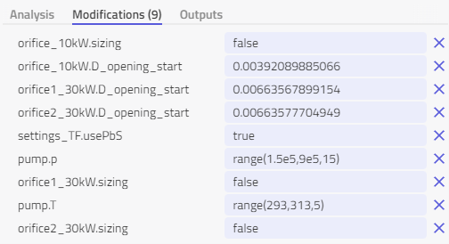
All modifications are the same as in experiment 2 but with an additional range( ) operator used such that the inlet temperature of the pump pump.T is varied between 293°K and 313°K or approximately 20°C and 40°C. The user must input values in Kelvin as SI Units have been enabled. This experiment is contained within the predefined list of experiments as Experiment 3 - Flow Simulation - dp_pump and T_pump Sweep.
The experiment contains two range( ) operators for two different parameters. The pressure boundary will be simulated over 15 values and the temperature value over 5 which means that the total number of executions that will be carried out is 5x15 = 75. A convenient way to visualize this domain exploration is to create a surface plot which can be done directly in Modelon Impact. The steps for creating one which shows the influence of both the pump pressure pump.p and the coolant input temperature pump.T on the return temperature at the merging junction staticJoin.join.T_mix are outlined below:
- Simulate experiment Experiment 3 - Flow Simulation - dp_pump and T_pump Sweep and rename the result to a fitting name.
- Select component staticJoin and drag calculated value staticJoin.join.T_mix onto the canvas. You should now see a 2D scatter plot.
- Select the component pump and drag the calculated value pump.pressureBoundary.T over the x-axis of the 2D scatterplot and drop.
- A new icon "3D" should appear in the top left-hand corner of the plot. Clicking it will create a surface plot. This caption can then be renamed to something more fitting.
The surface plot will then look something as follows:
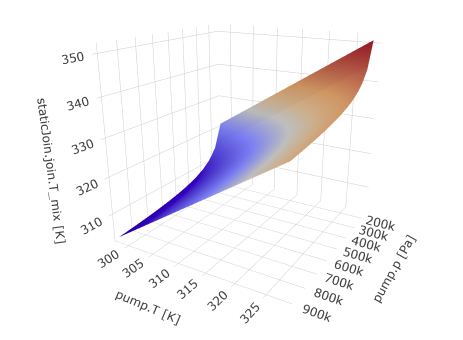
Figure 6: Newly created Surface Plot for Experiment 3 result - return temperature over a range of values for pump pressure and inlet temperature.
There exists a linear relationship between the pump inlet temperature and return temperature as is to be expected. The same non-linear relation between pump pressure and return temperature is also depicted here.