Enhanced Turbojet Multi-point

Introduction🔗

Classic cycle design relies on an on-design simulation at the design point. Afterward, the performance of the gas turbine can be computed on many other operating points using off-design simulation. However, the sequential process of defining the design parameters, computing performance on key operating points and going back to change the design parameters until all goals are met can be tedious. For complex cycles, it is also not always obvious how to change design parameters to satisfy potentially conflicting goals. Multi-point design, therefore allows a user to concurrently include an on-design model and several off-design models in a single experiment. The models are interconnected to use consistent sizing information, and design rules as well as control laws can be used to couple them.

Modelon Jet Propulsion Library provides models and utilities for the multi-point design of jet engines. These can be connected directly to other Modelon libraries that are part of Modelon Impact Pro.

Before we start🔗

You will need approximately 40 minutes to finish all tutorial steps.

What are we building?

This application is designed as a workshop, where we will expand the turbojet model created in the basic turbojet tutorial into a multi-point setup. The resulting model will roughly resemble the famous GE J85 from the 1950s, and we can use different design rules to size it across several operating conditions.

You will learn how to:

Prepare single-point experiments to support the setup of the multi-point model
Automatically generate a draft multi-point model
Expand the draft into a full multi-point model
Run it by reusing previously converged single-point steady-state solutions

Preparation🔗

We recommend structuring multi-point models in a specific way.

The baseline model is stored with the name Baseline. It contains the physical component model instances such as the compressor and turbine without any controls.
The controlled single-point model is saved with the name Controlled. It extends from the baseline model and adds controls and aggregation components.
The single-point model prepared for use as a sub-model in the multi-point setup is called SubModel. It also extends from the baseline model and adds inputs and outputs to feed data from the multi-point level.
Different multi-point setups are stored in sub-packages with meaningful names.

You can find an example of this structure for a more complex problem in the Jet Propulsion Library at JetPropulsion.Experiments.GearedTurbofan.MultiPoint.

With the modeling you did in the basic tutorial, you have already generated the first two models. For simplicity, the basic turbofan tutorial did not force the user to distinguish Baseline and Controlled models. However, this distinction is strongly recommended for this tutorial. Please split the turbojet model as described here in case you bypassed this before.

This tutorial covers a multi-point design of a conventional turbojet. If you implemented the bonus section of the basic tutorial, use the model you saved before adding electrification components or remove them from your experiment (if you did not create the copy).

** We are ready to build the multi-point setup now!**

Sub-model🔗

Previously, you ran on- and off-design simulations with the controlled model. We will now create a single-point model variant that is controlled externally, and can thus be included in the multi-point setup later on.

Creating it and providing outputs🔗

Adapt the sub-model from the previously created controlled model as follows.

Duplicate the controlled model Controlled by right-clicking it in the left pane and selecting Duplicate to. Enter SubModel as the new name.
We want to keep the aggregation utility cycleProperties processing thermodynamic station data. However, we must now provide the data to the outside from this model to enable integration in the multi-point setup. Therefore, delete the burner control block.
Drag the yellow bus connector JetPropulsion.Basic.Interfaces.Summary into the model. This is the bus we intend to use for making the cycle data available on the outside. Right-click it in case you want to rotate, move or resize it.
Connect the yellow bus connector of the aggregation utility cycleProperties to the newly created bus connector.

Your model should now look as follows.

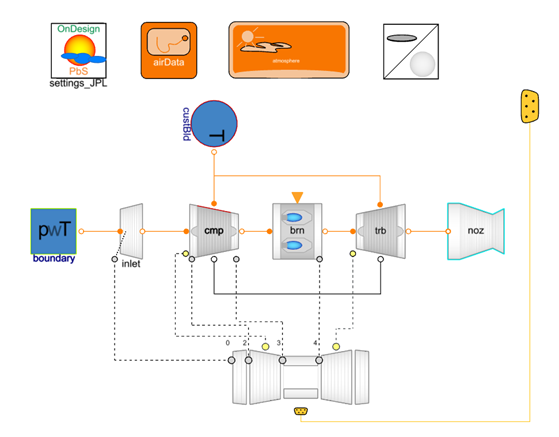
Receiving inputs🔗

Operation inputs🔗

Now add the first inputs from the multi-point level. They define how to operate the turbojet, e.g., how much fuel to inject at any condition.

Operational inputs are colored orange. Drag two such inputs into the model from
```
JetPropulsion.CyclePerformance.Control.Interfaces.OperationInput
```
Name the inputs far (for fuel-to-air ratio) and fracwBldCool (for the fraction of turbine cooling bleed flow).
The burner already has an input connector from the controlled model. Double-check that the burner is set to receive FAR at this connector by confirming that switchBurn is equal to FAR. Then connect far to the input u of the burner brn.
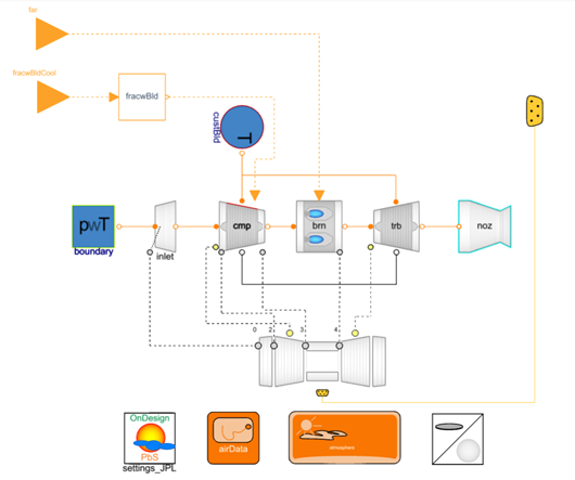
Next, we also set up the compressor to receive bleed flow fractions from external. To do so, navigate to the compressor parameterization in tab Bleed. Check the parameter fracwBldInputPrscr to receive all bleed flow fractions via input connector fracwBldInput.
Obviously, we have three bleed flow fraction for this compressor but only a scalar input on bleed flow fraction for turbine cooling that we want to prescribe from the multi-point setup. Therefore, drag the utility model JetPropulsion.CyclePerformance.Control.Compressor.Expanders.Bleed.DualCooling1PlusCustomer to the model canvas. As the name suggests, it expands the scalar cooling information to two cooling flows (for one turbine) and one customer bleed flow.
Connect the utility input to the operation connector fracwBldCool and the utility output to the compressor input connector fracwBldInput. Make sure to select the colon ":" to connect all components of the vectorized connectors!

Your model should now look as follows.

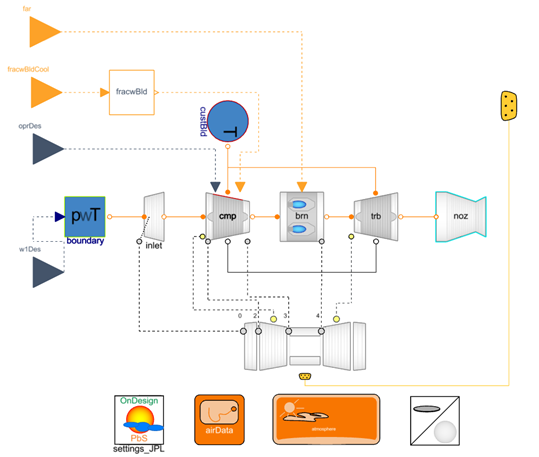
Sizing inputs🔗

Many sizing conditions can be established locally on the component level even in a multi-point model (turbine and nozzle sizing for instance). However, some sizing inputs are prescribed from the multi-point level, too (overall pressure ration for instance). We now add these to the sub-model.

Sizing inputs are colored dark blue. Drag two such inputs into the model from
```
JetPropulsion.CyclePerformance.Control.Interfaces.SizingInput
```
Name the inputs oprDes (for overall pressure ratio at design) and w1Des (for the mass flow rate at station 1 at design).
As the simple turbojet only has a single compressor, there is no need to break OPR into individual factors. We can use it directly to define the compressor design pressure ratio. Open the compressor parameterization, tab General and enable prDesInputPrscr when the sub-model is in on-design mode. Do this by writing settings_JPL.onDesign into the parameter field (expand it if necessary). Then connect oprDes to the input prDesInput of the compressor.
Note that also the sizing input connectors should be conditional to avoid misinterpretations of the model diagram. Currently, this manipulation has to be made in the code editor, so switch to code view. Press Ctrl+F to search for the name of the two connectors oprDes and w1des. You should find hits before the Modelica keywords equation. Directly after the connector names, write if settings_JPL.onDesign. Your two code lines should now look like this:
```
    JetPropulsion.CyclePerformance.Control.Interfaces.SizingInput oprDes if settings_JPL.onDesign annotation(/* ... */);
```
```
    JetPropulsion.CyclePerformance.Control.Interfaces.SizingInput w1des if settings_JPL.onDesign annotation(/* ... */);
```
Press the Check syntax button, and Save if no errors are reported. Switch back to diagram view.
Open the boundary parameterization, tab General. Again, enable useInputw when the sub-model is in on-design mode by writing settings_JPL.onDesign into the parameter field (expand it if necessary). Then connect w1des to the input commandSignal of the boundary.
Finally, we must also enable the prescription of polytropic efficiency only for design points. Therefore, open the General tab of both the compressor and turbine parameterization. For each, set effPolyPrscr to settings_JPL.onDesign (again, expand the checkbox if necessary).

Your model is now ready for automatically generating the draft multi-point model and should look as follows.

Tip

You can also add an icon to your sub-model such that it is visualized in the multi-point setup later on. In this release, there is no graphical interface to do this yet. You can however open the code editor and paste the following code into the penultimate code line after annotation( (note the opening parenthesis "(").
Icon(graphics = { Bitmap(extent={ {-120,-100},{140,100} },fileName="modelica://JetPropulsion/Resources/Images/Outline.png"),Text(extent={ {-20,-40},{100,-60} },lineColor={68,84,106},textString="%name") }),
This will include a default image and instance name as text.

Multi-point model🔗

We will now create the multi-point model. This has two main steps. First, we automatically create a draft model with the sizing link between on-design and off-design points. This draft is then edited manually to complete the multi-point setup.

Generating the draft🔗

Create a new package that you use to structure the models for this particular multi-point setup. Typically, choose a meaningful name describing your multi-point scheme. Here, simply call it MyMultipoint or ConstantT4inCrz.
Double-click in the left pane the sub-model you created previously to select and view it.
Go to the Experimentation mode (by clicking on it).

Select Jetpropulsion (B1): Generate Multi Point custom function by hovering your mouse over the run button.

Adjust all parameters of the custom function.
1. For name_ondesign, enter sls (Sea Level Static). This will be the name of the instance of the sub-model in on-design mode.
2. Set name_offdesign to crz (cruise conditions). This will be the name of the instance of the sub-model in off-design mode. The custom script will only generate one instance of the off-design model but you can later copy this to create any additional number.
3. For model_name_multi, make sure to enter a suitable name for the model being generated. Here, %package(0)% refers to the package the currently selected model Controlled is in. You should then provide the name of the package you use to organize the multi-point models (MyMultipoint or ConstantT4inCrz per above). Finally, append the name of the model being generated such as Generated. The complete argument for model_name_multi should therefore be %package(0)%.MyMultipoint.Generated.
Run the model generation as usual. You can then load the generated model.

Note

In this release, the model generation is only supported for models created one-by-one. If the generated model is not loaded with the dialog shown above, then you have likely duplicated a complete package instead of creating models one by one. To avoid this, first create the new package you want to duplicate, and then duplicate each model within the package one by one. Then, this issue will disappear.

Implementing the setup🔗

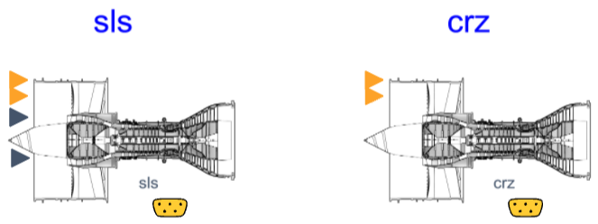
Initially, the model looks as follows. The on-design instance sls and the off-design instance crz are clearly visible.

Copy the generated model to a new model called Setup by right-clicking it in the left pane and selecting Duplicate to.
In the model canvas, create a second off-design point by selecting the crz off-design model and choosing Duplicate. Rename it to toc.
Set up the conditions of all sub-models by right-clicking them and choosing Inspect component. You can now see the inside of the sub-model in the context of the multi-point setup.
1. Inspect the on-design sub-model sls and confirm that altitude alt_par and Mach Number Mn_par are both zero. Also, the usePbS and onDesign flags should be active.
2. Inspect the off-design sub-models toc and crz and set altitude alt_par to 35,000 ft and Mach Number Mn_par to 0.78 for both. Confirm that the onDesign flag is inactive.
We now assume that we do not know the design overall pressure ratio (OPR) but want to prescribe the cruise OPR to be 6 to yield a balanced design. Therefore, drag and drop the instance of
```
 JetPropulsion.CyclePerformance.Control.Compressor.OverallPressureRatio
```
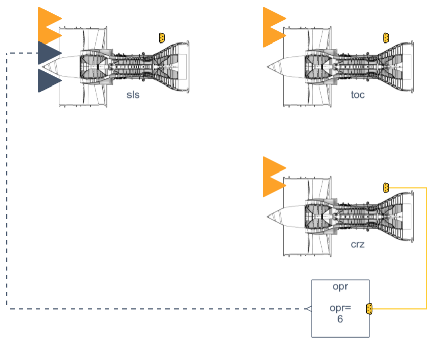
onto the canvas. This allows us to find design OPR from OPR in one of the points. To choose which OPR to consider, connect the yellow bus connector to the case for which you want to prescribe OPR. In our case this is the model crz. Select the utility opr and press Shift+H in case you want to flip it horizontally. Also, connect the output oprDes of the utility to the design point model sls input oprDes, and enter the threshold 6 for oprPrscrPar in the utility opr.
Your model looks as follows.

We also wish to prescribe the burner outlet temperature T4 in cruise, so we drag another utility
```
JetPropulsion.CyclePerformance.Control.Boundary.FlowRateFromBurnerOutletTemp
```
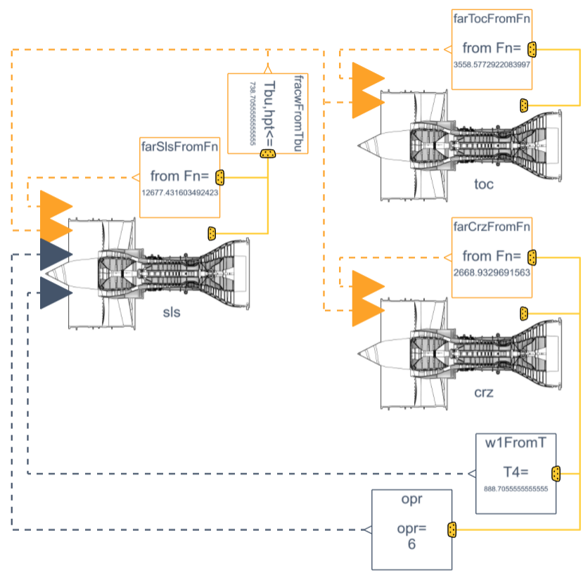
onto the canvas. Connect it to the summary connector of the cruise model crz, and the design point air flow rate w1des of the design point model sls. Set the target T4PrscrPar to 1140 °F in the utility w1FromT. We have now defined all sizing rules for the turbojet.
For the turbine cooling bleed flow computation, we create an instance of
```
JetPropulsion.CyclePerformance.Control.Compressor.FlowFractionFromTurbineBladeTemp
```
in the model. In our case, we will compute cooling bleed flows for the hottest condition (SLS), and propagate these into all conditions. Connect the yellow summary connector of the utility fracwFromTbu to on-design model sls. Set the maximum uniform blade temperature TbuMaxPrscrPar to 870 °F. Connect the output fracwBldCool to all three sub-models sls, toc and crz.
Finally, we must create one instance of
```
JetPropulsion.CyclePerformance.Control.Burner.FarFromNetThrust
```
for each sub-model to find the amount of fuel to be injected in the respective conditions. We do this by prescribing the net thrust to be generated. Establish thrust thresholds with this utility per table.

Condition
Sea-level static (SLS)	2,850 lbf (12.7 kN)
Top of climb (TOC)	800 lbf (3.6 kN)
Cruise (CRZ)	600 lbf (2.7 kN)

The model is now complete.

Simulation🔗

All models were set up now and we can start simulating the multi-point problem.

Review single-point experiment results🔗

As we will reuse results from single-point experiments to initialize the multi-point problem, we will start by reviewing these. Note that this is not strictly required as simple models such as the turbojet are easy to converge. However, we apply this process such as to describe a generic process that can be used conveniently for most kinds of gas turbine models.

Open the controlled single-point experiment by double-clicking it in the left pane. It should be called Controlled and be stored one level up of the MyMultipoint package you worked on last.
Switch to the result mode by clicking Results (or any custom result name) in the top pane.
Review that you retained results at least for SLS and TOC, and that you named them as suggested.

Tip

For more complex models, it is recommended to have one single-point result for each sub-model instantiated in the multi-point setup.
To estimate cruise results in a single-point model you can reduce the prescribed burner outlet temperature for an off-design simulation or prescribe net thrust in the burner (see switchBurn parameter).
You can create off-design results as described before with custom function A1 or with custom function A2 (in case of convergence is not achieved when reusing previously converged results via the Advanced parameter initialize_from). Custom function A2 implements essentially the same functionality as A1 but additionally takes intermediate convergence steps. (The key boundary conditions used in the previously converged results are extracted from the initialize_from argument. Then, the model is initialized with guesses based on initialize_from and the corresponding boundary conditions. The boundary conditions the user is interested in from the current setup are not applied right away. Instead, increments of boundary conditions are found based on user input to custom function A2, and the boundary conditions are adapted incrementally towards the values of interest for the given case while converging the model at all intermediate boundary conditions.)

Define guesses for utilities🔗

Previously converged single-point results can automatically be reused to initialize sub-models in a multi-point experiment. However, most of the utility blocks instantiated in the multi-point experiment also introduce unknowns that the solver iteratively converges. Therefore, these also should be initialized.

In the parameterization of utility opr, set the OPR start value oprDesStart to 7 as the default targets state-of-the-art geared turbofans.
In the parameterization of utility w1FromT, enter a guessed airflow rate at the design point w1DesStart of 44 lbm/s as the default also targets larger turbofans.

Tip

In this example, we only adapt the guesses for which the defaults (targeting today's turbofans) are inappropriate for the small turbofan example. For more complex models, it is recommended to enter start values for each such utility block on the multi-point experiment. These can usually be found easily in the single-point results, too. For instance, if the net thrust of your single-point simulation roughly matches the net thrust you impose for the same condition in the multi-point experiment, then you can use the fuel-to-air ratio (FAR) from the single-point results of the controlled model. Similarly, all other potentially required guesses such as design fan pressure ratio, design bypass ratio and so on can be accessed conveniently. Whether this is required depends on the complexity of the plant model you built and its convergence robustness.

Simulate it!🔗

For the multi-point experiment Setup, go to the Experimentation mode.

Select Jetpropulsion (B2): Simulate (Multi Point) custom function by hovering your mouse over the run button.
Adjust all parameters of the custom function.
1. Parameter model_name_single is the name of the single-point experiment whose results you want to use to initialize the multi-point model. All result names you want to use will have to appear when you select this model. Keep the default %package(1)%.Controlled if you stored the controlled single-point experiment in the recommended package. Operator %package(1)% refers to the package one level up of the one currently selected.
2. Parameter mapping contains the information describing how to reuse named single-point results to initialize instances of the sub-model in the present multi-point experiment. The mapping is provided as an array of instance name and result name pairs. The entry 'toc':'TOC' for instance means that the sub-model instance toc shall be initialized with results you called TOC. If you want to initialize the sub-model toc with results TOC second try or CRZ then use entries 'toc':'TOC second try' or 'toc':'CRZ' respectively. It does not cause any harm if you list entries for sub-model instances that do not exist in the current model (e.g., for the turbojet you can include an entry 'rto':'RTO' despite there is no sub-model called rto).
  In our experiment we wish to initialize the sub-model instance sls with results SLS. However, for sub-model instances toc and crz we do not distinguish conditions carefully and wish to initialize both with results called TOC. Therefore, enter the array {'sls':'SLS', 'toc':'TOC', 'crz':'TOC'} for this argument.
3. For store, keep the default value true such that a model initialized with the found solution is stored in the model repository.
4. Argument model_name_init can also remain at the default. Like this, the postfix Initialized will be attached to the name of the present multi-point experiment when storing the results.
Run the model generation as usual. You can again load the generated model and browse the multi-point results.

Congratulations, you have successfully designed a turbojet with a multi-point setup!

Continue by reviewing a more representative multi-point setup for a geared turbofan model in the Jet Propulsion Library. It is available under JetPropulsion.Experiments.GearedTurbofan.MultiPoint. Refer to the following article.