Mechanics Modeling Basics🔗
This section will explain the basic concepts that are necessary to understand when you are doing mechanics modeling in Modelon Impact.
Types of models🔗
There are 3 main types of mechanics models in Modelica:
- Translational
- Rotational
- Multibody
In addition, in Modelon Base Library, there is a package - Rotational3D that combines a 3D multibody connector with a Rotational connector. This is useful when modeling rotating parts in a 3D context such as wheels, drivelines, and rotors.
Connectors🔗
A mechanics connector, like other Modelica connectors, has potential and flow variables. For translational, they are position and force, for rotational they are angle and torque. For MultiBody, the connector is a bit more complicated, it contains position, orientation as well as force and torque, all in 3 dimensions. In principle, it works the same as the 1D connectors, though the Modelica code and compiler techniques behind it are more complex. But we don't have to worry about that now.
When two mechanics connectors are connected, it implies a rigid coupling. This means the position/angle/orientation is constrained to be the same, and the forces/torques should sum up to zero. This is also true if more than two connectors are connected, the forces/torques in all connectors in a connection set need to sum up to zero.
First model🔗
We will build a very simple model of a mass and a spring. We need the following components:
- Modelica.Mechanics.Translational.Components.Fixed
- Modelica.Mechanics.Translational.Components.Mass
- Modelica.Mechanics.Translational.Components.Spring
Add these three components and connect them in series, Fixed -> Spring -> Mass.
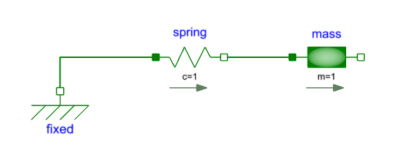
Set the spring stiffness (spring.c) to 1 and the mass (mass.m) to 1.
Now run the simulation and look at the position of the mass (mass.s).
Note that the mass isn't moving. We can further look at the force in the spring (spring.f), and see that there is no force in the spring. So the system is initialized in equilibrium.
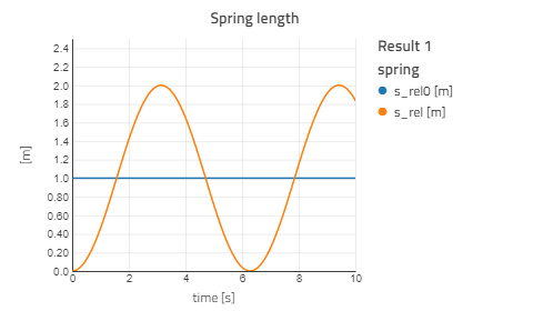
To excite some motion in the system, we can set the unstretched spring length (spring.s_rel_0), to 1. This means the spring will give zero force when the relative displacement (spring.s_rel), is 1. Since we still initialize with s_rel = 0 we are no longer in equilibrium at the start of the simulation.
Sign conventions🔗
For the translational 1D components positive displacement is defined from flange_a to flange_b. A positive force/torque moves a mass/inertia in the positive direction (from flange_a to flange_b). Arrows on the translational component icons indicate this sign convention. This sign convention holds true for rotational components as well.
In the spring-mass model above, we will see what happens if we flip the spring:
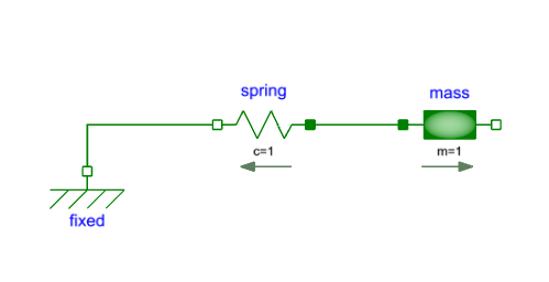
Note
The arrow now goes from right to left.
Now, if we look at the relative displacement in the spring, we see the same thing as before:
However, if we compare the mass position to the previous model, we see how the model is different:
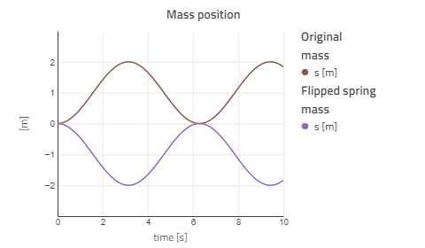
The spring itself still has the same parameters, s_rel0 = 1, meaning that the unstretched spring length is 1, and the spring "wants" to be at s_rel = 1. This doesn't change when we flip the spring. What does change is s_rel, since it is defined as the displacement from flange_a to flange_b, meaning that the mass will move in the opposite direction.
States and state selection🔗
This section introduces the concept of states and an Impact tool for understanding how a mechanics model is solved. For mechanical systems, the degrees of freedom (DOF) are essentially the directions that the system or parts of the system can move without breaking. The 1D translation example above has only one degree of freedom.
A rigid body in space has 6 - three translations, and three rotationals.
The minimal set of variables needed to uniquely define the state of the system are called state variables. For the oscillating mass system above, we know that it has one degree of freedom (translation). The system can be fully defined if we know the position of the mass and its velocity. Now we will check that it is indeed the case by compiling and simulating the model with the generate_html_diagnostics option turned on.
This can be found in Settings > Execution > Compiler Options > generate_html_diagnostics.
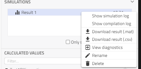
Simulate the model after activating the generate_html_diagnostics option and in the result model select Result 1 > View diagnostics.
Expanding State variables in the generated report shows mass.s and mass.v as states:
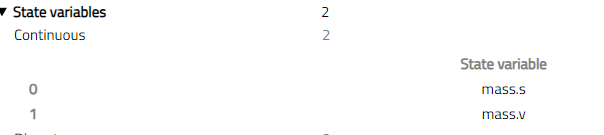
One thing to keep in mind while we move forward and eventually to 3D mechanics is that with one degree of freedom, we require two states to define the system, this principle will be consistently applied to all models.
For the models covered in this tutorial and the simple spring-mass example, the default settings in Impact show predictable states. There are certain cases where we might want to select different states. Most mechanics components which contain variables that can be defined as states, have a stateSelect flag for example under the Advanced tab for mass:
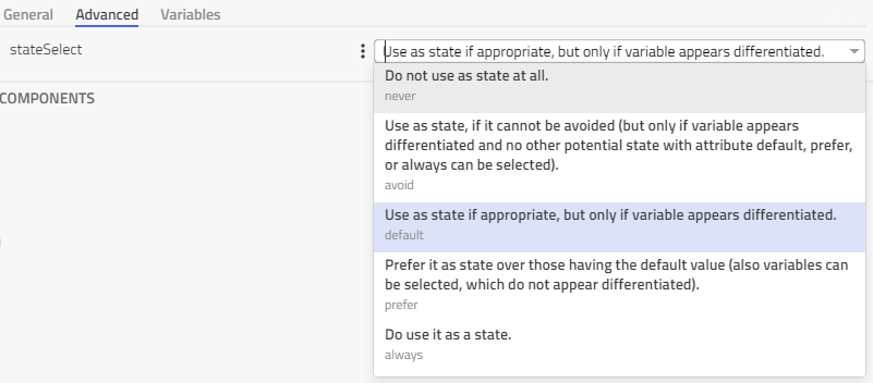
This parameter can be used to assign priority to certain states in a model over other possible ones with the order always having the highest priority and never the lowest.
Inertial effects are based on motions relative to the absolute (inertial) system. An example is the Modelica.Mechanics.Translational.Components.Mass component:
  v = der(s);
  a = der(v);
  m*a = flange_a.f + flange_b.f;
It should be kept in mind that the variables s is the absolute position of the mass. For applications where the absolute position is unbounded (for example: a rotating inertia in a vehicle drivetrain), it is preferable to use relative states instead. Further explanation can be found in Modelica.Mechanics.Translational.UsersGuide.StateSelection.
Rigid vs Compliant🔗
Kinematic components define the relationship between flange_a and flange_b. This means that the position of flange_b can be uniquely defined from the position of flange_a and the internal properties of the component. If one flange is constrained, the other is also constrained. In other words, kinematic components introduce constraint equations between two components. A gear (Modelica.Mechanics.Rotational.Components.IdealGear), is an example where the ratio defines the rotation of one flange relative to the other:
phi_a = ratio * phi_b;
Compliant components, on the other hand, are defined by the motion of both flanges, and some force/torque is applied as a result. The Spring component from the above example generates a force based on the relative motion of its two flanges:
f = c * (s_rel - s_rel0);
As a result of this dependence on the position of both flanges, we need the motion of the two flanges as state variables so that the behavior of the system can be described. Compared to the kinematic components, the compliant components require states to define a system and do not introduce constraint equations. When one end of a compliant component is fixed (like the example at the beginning) there are no states for the fixed end as its motion is fully defined.
Using this information about kinematic and compliant components, the total number of states required to describe a 1D system can be calculated and explicitly defined.
1D Kinematic model🔗
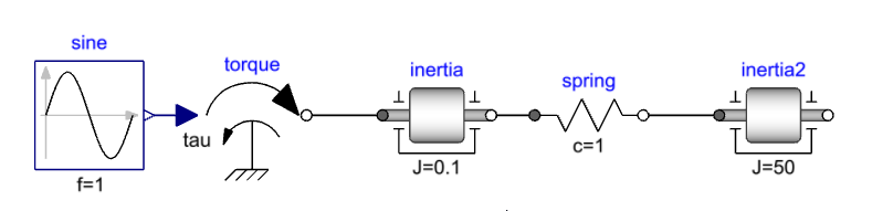
We can now build a 1D rotational mechanics model which shows these principles using the following components:
- Modelica.Blocks.Sources.Sine
- Modelica.Mechanics.Rotational.Sources.Torque
- Modelica.Mechanics.Rotational.Components.Inertia
- Modelica.Mechanics.Rotational.Components.IdealGear
Connect these components as shown below:
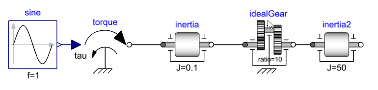
Set the following parameters:
- Frequency of the sine input, sine.f = 1.
- Moment of inertia for first inertia, inertia.J = 0.1.
- Gear ratio, idealGear.ratio = 10.
- Moment of inertia for second inertia, inertia2.J = 50.
Starting from the torque source, we are defining the torque input to inertia.flange_a. The torque balance equation inside the inertia component is used to fully define flange_a and in turn the flange_b rotation. Since the idealGear is a kinematic component, it fully defines idealGear.flange_b and in turn inertia2.flange_a.
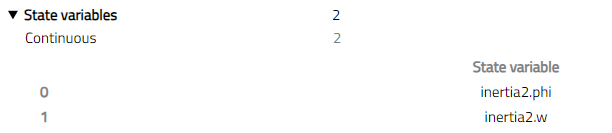
Only two states corresponding to 1 degree of freedom are required to fully define the system: the angle and angular velocity of one inertia. Simulate the model after activating the generate_html_diagnostics option and in the result model select Result 1 > View diagnostics.
In the HTML report, the selected states are shown under the State Variables section. Expanding it shows that inertia2.phi and inertia2.w are being used as states in this case.
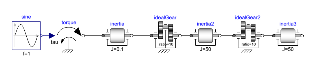
Now we have seen that kinematic components do not require states to define the relationship between their connectors, we can add more of them, and still, two states can fully define the system. Add one more idealGear and inertia to the model by copying idealGear and inertia2.
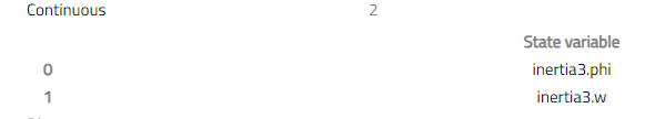
Simulating this and checking the states again shows that two states are selected, inertia3.phi and inertia3.w in this case.
1D Compliant model🔗
Now we will introduce compliant components in our model. Update the first kinematic model by replacing idealGear with Modelica.Mechanics.Rotational.Components.Spring. Set the spring stiffness (spring.c) to 1. Since the spring requires the rotation of both the flanges and calculates the resulting torque, the states are required on both sides of the spring.
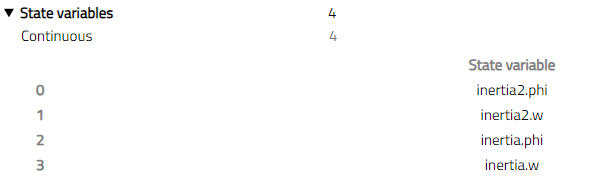
Simulating this model and checking the states shows that we now have four states:
- inertia.phi
- inertia.w
- inertia2.phi
- inertia2.w
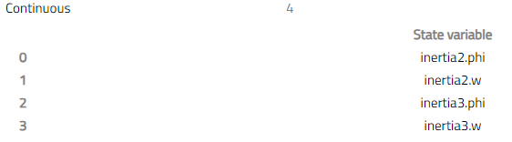
Kinematic and compliant components can be combined while following the same rules. Add an ideal gear and additional inertia to the model and simulate it again.
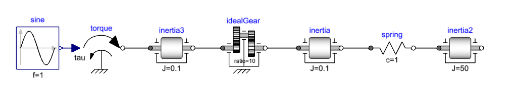
Two states are required to describe the kinematic chain like before (left of spring) and two more required from inertia2 to describe the system. We can see that the selected states are inertia2.phi, inertia2.w, inertia3.phi and inertia3.w.
3D Mechanics🔗
Positions and orientations🔗
The connector used to describe 3-dimensional mechanical components is called a Frame Connector. To fully describe an object in three dimensions, both position and orientation relative to a known reference are required. Each frame connector has a position and orientation (along with three forces and torques).
Compared to the case with 1D components, now there are 6 degrees of freedom that need to be defined. It should be noted that, unlike the 1D connectors, these d.o.fs are defined internally by more than just six sets of flow and potential variables. Despite this, the concepts from 1D modeling like state selection, kinematic, and compliant connections are still applicable. Connecting two frames defines their position and orientation to be the same. Now we will look at some kinematic multibody models.
Joints🔗
Primitive joints are used to allow relative movement in certain directions (degrees of freedom) while constraining the rest. The following primitive joints are available in the Modelica.Mechanics.MultiBody.Joints package:
- Revolute - 1 Rotational d.o.f. around an axis, hinge joint.
- Prismatic - 1 Translational d.o.f. along an axis.
- Universal - Two rotational d.o.f.s.
- Spherical - Three rotational d.o.f.s.
A joint will define the motion along some of the six degrees of freedom between its two frames(frame_a and frame_b). For example, the motion of the revolute joint is defined by the angle and angular velocity around the defined axis of rotation. Using the angle, and angular velocity as states fully define the frame_b with respect to frame_a.
For systems without closed loops (a frame is not connected to anything for the last component in the series), joints and bodies can be connected in any order. The exception is connecting the joints together, which doesn't make physical sense like connecting two sphericals in series. Connecting two revolutes with orthogonal axes is fine as it results into a universal joint.
Keeping how the motion is defined for a joint in mind is useful to model kinematic loop structures along with the fact that there are 6 degrees of freedom at each frame connector.
Force elements🔗
Like the 1D compliance components, a force element generates forces/torques based on the motion of its two frames and does not add constraints to the model. For example Modelica.Mechanics.MultiBody.Forces.Damper.
This also means that both frames of such a component need to be defined. This is usually done by defining relative states between frame_a and frame_b.
Rigid components🔗
Like the 1D kinematic components, the rigid 3D components define a relationship between the position and orientation (6 degrees of freedom, instead of one for 1D translation/rotation) between frame_a and frame_b.
For example Modelica.Mechanics.MultiBody.Parts.FixedTranslation adds a translation between frame_a and frame_b while keeping the same rotations. They are also used to add inertial effects and mass properties (Modelica.Mechanics.MultiBody.Parts.Body).
Building a simple model🔗
We will build a simple pendulum model using primitive components from the Modelica.Mechanics.MultiBody library. We need the following components:
- Modelica.Mechanics.MultiBody.World.
- Modelica.Mechanics.MultiBody.Joints.Revolute.
- Modelica.Mechanics.MultiBody.Parts.BodyBox.
Add these three components and connect them in series, World -> Revolute > BodyBox. Set the bodyBox frame_b position (bodyBox.r*) to {0.5,0,0}.
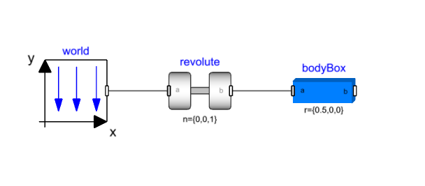
Run the simulation for 10 sec and view the animation by right-clicking on the canvas and selecting View 3D animation. Animation is available by default for multibody models when the Modelica.Mechanics.MultiBody.World component is used. The green arrow in the animation window shows the direction of the gravity vector, in this case negative Y axis. The bodyBox is initialized along the X-axis and oscillates because of its mass. Plotting the revolute joint angle shows this behavior.
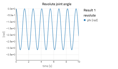
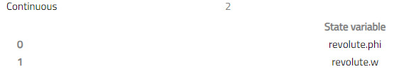
The revolute joint adds one degree of freedom between frame_a and frame_b which is the rotation in the Z direction. This rotation angle and its derivative fully define the system. The next component bodyBox is rigid with frame_b fully defined with respect to frame_a. If we look at the state variables for this model we can see that revolute.phi and revolute.w are the two states.
Add another pendulum🔗
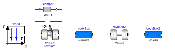
Next, we will add another revolute joint and bodyBox component to complete our double pendulum model. This can be achieved by copying the revolute and bodyBox and pasting it on the canvas. Connect the new revolute to the first bodyBox.
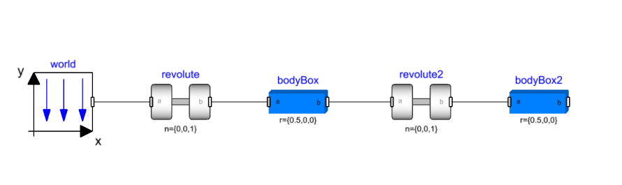
Now the second revolute joint is adding one degree of freedom between bodyBox.frame_a and bodyBox2.frame_a, defined by revolute2.phi and revolute2.w states which can be verified in the HTML diagnostics.
Just like the 1D kinematic model, more joints and bodies can be added to this chain. Each additional joint will introduce a number of new states, depending on which type of joint it is.
As long as we don't close the kinematic loop by leaving the frame connector of the last component in the series disconnected, we can add as many additional components as we like without issues.
Add damping🔗
Next, we will add some damping to one of the revolute joints. Since we want to add rotational damping and the 1D and 3D connectors are different in terms of the number of variables, we need a way of connecting the two. Joints with one degree of freedom (Revolute and prismatic) enable this by exposing 1D connectors along the direction of motion. For the revolute joint, this is done by setting the parameter useAxisFlange = true. This exposes two rotational flanges and the Modelica.Mechanics.Rotational.Components.Damper can be connected. Set the damping coefficient (damper.d) to 0.1 and simulate the model again.
Mechanisms and kinematic loops🔗
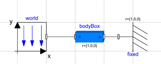
Unlike the pendulum example shown above, a majority of mechanisms are kinematic loops i.e. both ends are constrained in certain degrees of freedom. For example: a slider crank is constrained to rotate on the crank end and translate on the slider end. While it is possible to model such kinematic loops, some considerations need to be made as a consequence of a rigid connection adding 6 constraint equations which are too many when creating a kinematic loop. This results in redundant constraints, an example of which is a rigid body with two fixed joints as shown below. The bodyBox component is rigidly connected to the world which means bodyBox4.frame_b is fully defined. If we connect the fixed component to bodyBox, we are constraining the same 6 degrees of freedom as the world, which means these constraints are redundant. This concept also applies to kinematic loops, as explained below.
We can build a simple kinematic loop by connecting four bodyBox components as shown below:
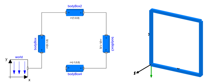
The model shown above simulates and produces the animation on the right but if bodyBox4.frame_b is connected to the world, which is equivalent from a system perspective, we get a compilation error:
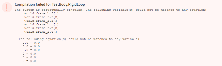
Since the bodies are rigid, the position and orientation of bodyBox4.frame_b are fully defined (starting from the world) and we add more constraints by adding the last connection. Removing any one of the connections gets rid of these redundant constraints and the system is uniquely defined.
Such errors can be encountered when closing a kinematic loop in 3D mechanics and the following section explains how to identify and deal with this using a four bar linkage example.
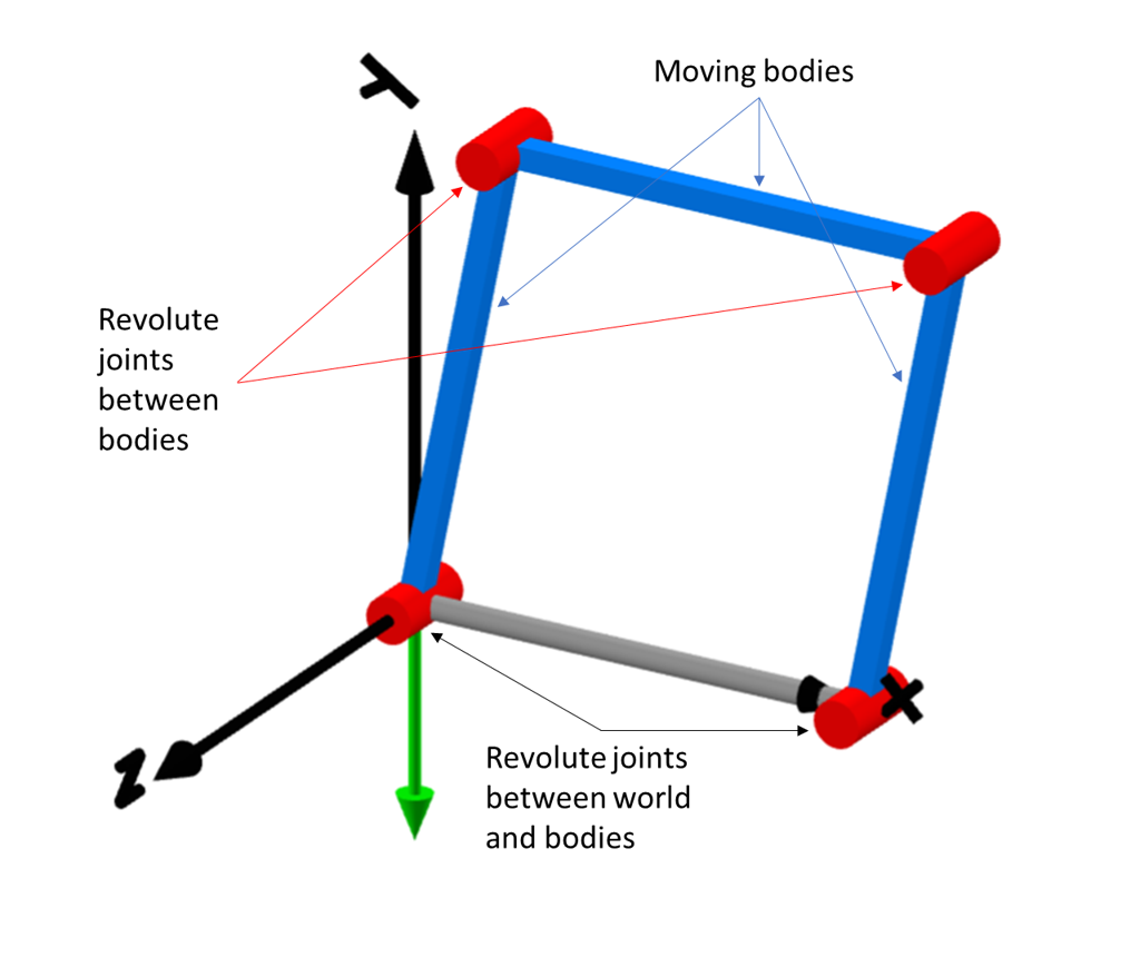
Four bar linkage and the first example🔗
A four-bar linkage is a mechanism that forms a single loop made up of three moving parts. We will be working with a planar version of this mechanism where two revolute joints connect two parts to a fixed reference (world) and two more revolute joints connect the third body to these two bodies. All of the joints have the same axis of revolution and are located in the same plane (X-Y in the example below) resulting in planar motion of the mechanism defined by input to one of the joints.
Intuitively, all four revolute joints appear to be the same so we will create a four bar mechanism using the following components:
- Modelica.Mechanics.MultiBody.World.
- Modelica.Mechanics.MultiBody.Joints.Revolute.
- Modelica.Mechanics.MultiBody.Parts.BodyBox.
- Modelica.Mechanics.MultiBody.Parts.FixedTranslation.
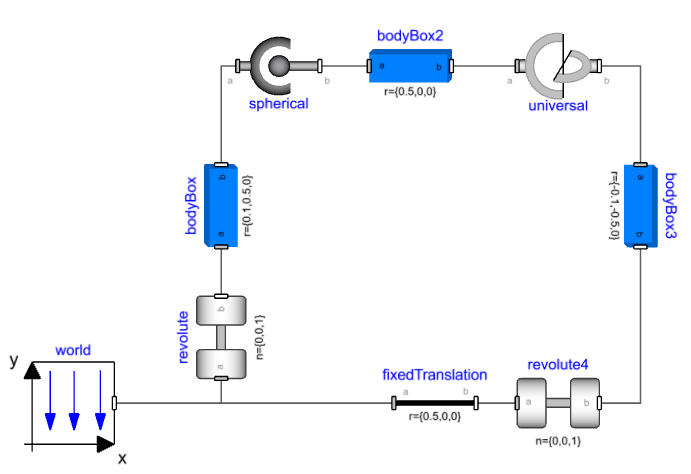
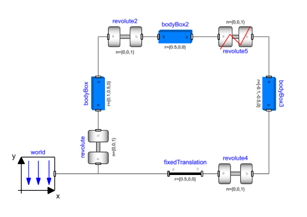
Connect four revolute joints and three bodyBox components as shown below:
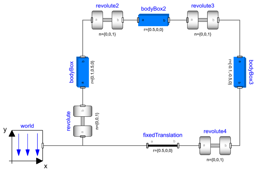
Set the translation parameters as:
- bodyBox.r = {0.1,0.5,0}
- bodyBox2.r = {0.5,0,0}
- bodyBox3.r = {-0.1,-0.5,0}
- fixedTranslation.r = {0.5,0,0}
If we try simulating this experiment we get a compilation error:
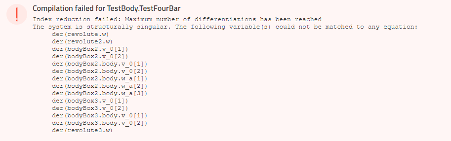
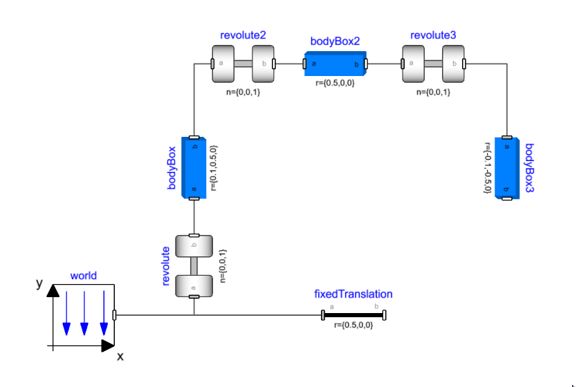
This error points to the number of constraints exceeding the number of variables available in the frame connector. If we remove one of the revolute joints like below we have essentially turned our model into a tree - like the double pendulum. It translates and simulates with states in the three revolute joints.
Now that we have identified that we have too many constraints, we can look at removing the redundant constraint equations. We know that the bodyBox components are rigid and have 6 equations inside them while there are different joints available that can have less than 5 constraint equations. We will look at replacing some of the joints to get rid of the additional constraints.
Removing redundant constraints in planar loops🔗
For the specific case where the movement of the bodies is restricted to one plane (XY plane in our case) i.e. planar loops; a revolute joint is available which has 2 constraint equations instead of 5 (Modelica.Mechanics.MultiBody.Joints.RevolutePlanarLoopConstraint).
Since the positions of each frame are in the plane orthogonal to the rotation axes of the revolutes and the revolutes all have the same axis of rotation, we can simplify one of the revolutes to the constraint that the x and y positions of the two frames need to be equal.
We then assume that the two z positions are the same (which is true if the loop is indeed planar) so we don't need to add that constraint. The revolute will not transfer any torque around the rotation axis.
Then we're left with the torques around the x - y axis, and the forces. The out-of-plane force (z) and torque (x,y) are assumed to be zero as these are not uniquely defined in a loop like this, so zero is a good guess as any. The reaction forces are therefore assumed to be in the x,y-plane.
Replacing one of the revolutes with this joint successfully compiles and simulates the model. Note that for this kinematic loop, the angle and angular velocity of one joint are required to define the system which can be verified in the diagnostics to be revolute.phi and revolute.w.
Removing redundant constraints using standard joints🔗
Taking a look at revolute2 in the mechanism, it is oriented in the same direction as revolute. Out-of-plane motion for bodyBox2 (Rotation about X and Y axis) is already constrained by revolute. We can think of replacing the revolute joint with a joint that can allow these movements and remove the corresponding constraint equations while maintaining the kinematic behavior.
A spherical joint does not have constraint equations on the orientations between its two connectors, so it can remove the X and Y rotation constraints while allowing the same Z rotation that revolute2 presented.
Next, if we consider revolute3, it constrains the same out-of-plane motion as well. Replacing this with a spherical joint will remove the constraints on X and Y rotation but will introduce an additional spin degree of freedom for bodyBox2 (around its own axis). Using a universal joint with its axes set to the Y and Z direction it gets rid of this additional degree of freedom while removing the two orientation constraints. Replacing revolute2 and revolute3 with a spherical and universal joint (n_a set to {0,0,1}) respectively gives a model that translates and simulates successfully.