Create a Model

Introduction

The purpose of the tutorial is to show the typical steps for building a model, running an experiment and reporting results using Modelon Impact.

Modelon Impact is a web-based modeling and simulation environment. Access and use of the tool is through the web browser.

About the tutorial

The time to complete the tutorial is approximately 20-30 minutes.

The tutorial shows how to build a small fluid system consisting of two open tanks connected by two pipes.

Going through the tutorial will teach the essential skills of working in Modelon Impact. The purpose is to show how Modelon Impact works using the Graphical User Interface and libraries.

You will learn how to:

• Create a new workspace
• Build a model by adding and connecting components
• Set component properties also known as component parameterization
• Set simulation settings also known as experiment settings
• Run a simulation also known as running an experiment
• Display results by plotting variables
• Add views and stickies for diagram animation and analysis

Pre-requisites

In order to perform this tutorial Modelon Impact, installed on desktop, on-prem or cloud must be with a valid license.

Create Workspace

Models are built within a workspace. The workspace has to be created and named. A workspace is where a user keeps models, libraries and other resource files used for a particular project. One workspace can contain multiple models that use different libraries.

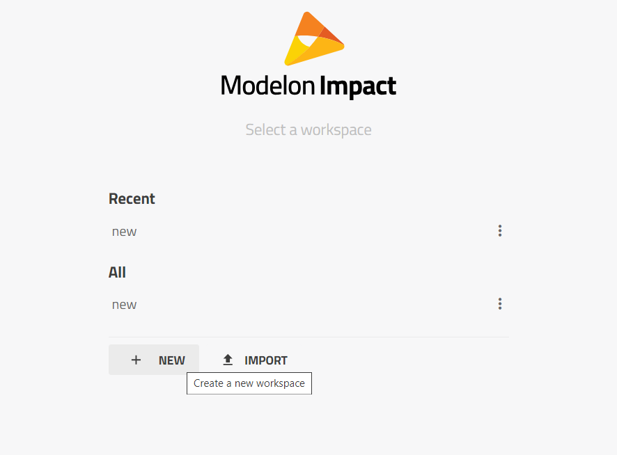
1. A workspace is created and opened from the welcome page.
2. Click the New button to create a new workspace.

Graphic: Creating workspace

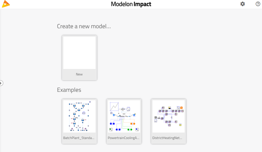
3. Give it the name "my_workspace". This will create a new workspace and open the workspace panel.

Graphic: New workspace landing page

4. For Modelon Impact desktop application, the workspace is stored locally on your computer. Learn more.

You are now ready to create your first model in your workspace!

Create a top level package

1. Once my_workspace is set up open the workspace panel.
2. You will notice a default Project already created.

Note

The Projects are editable and all data is stored there.

3. Click on the + button in project to open up the Create new class menu and create a new top level Modelica Library/Package and name it as my_workspace.

GIF Create a top level package

Build model

Modelon Impact is a model-centric tool. The model you build and work on is at the center of all operations performed such as experimenting and analyzing performance.

In Modelon Impact, a model is created inside a container/package called Project. The components which make a model are dragged from a library (located in the workspace browser to the left) into the model canvas. Connecting and parameterizing the components makes the system ready for simulation.

The aim is to build a model consisting of two tanks connected by pipes by using components from the Modelica Standard Library, also known as MSL.

Each tank is placed at different heights where the initial water level is lower in tank2. The expected result is to finish up with the same water level in both tanks.

Create a new model

1. Open the left sidebar, known as the Library Browser (Workspace Panel).
2. Initially a default container Project will be created.
3. Click on the + button in project to open up the Create new class menu and create a new top level Modelica Library/Package and name it as my_workspace.
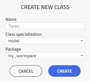
4. Right click on my_workspace and click New Model.
5. Name the new model Tanks and press Create. By convention, class names should start with an upper-case letter.

GIF Create a model

Can also create a new model by clicking new on the landing page.

Note

Learn more about the Class specialization option

This creates a new empty model named Tanks within your Workspace library.

Tip

Right-click on a library package and choose "New model" is a quick way to create a new model.

Add components

The next step is to find specific components and place them on the canvas. You will only use components from the Modelica Standard Library.

You will use the following model components:

 Modelica.Fluid.Vessels.OpenTank

 Modelica.Fluid.Pipes.StaticPipe

 Modelica.Fluid.System

1. Find the components within the Modelica library folder. The Library filtering function can be used.
2. Add them to the model canvas.

Graphic: Adding Components

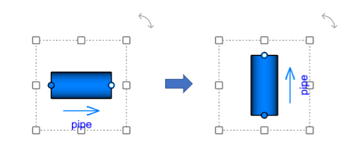
3. Select and rotate the pipe using the right top rotating mark.

Tip

Click on and choose Shortcuts & Controls showing how to efficiently navigate the canvas.

Connect components

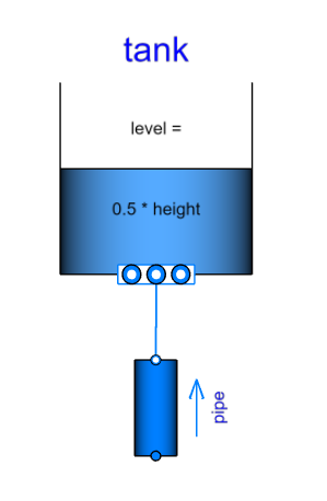
1. Connect the tank and pipe together with the left mouse button from the bottom of the tank to the top pipe opening.

   

Tip

Compatible connectors are highlighted when you start dragging the connection line.

Note

The shape of the connection line can be edited by dragging at either the line or the corner point, once the connection is done.

Set component properties

The next step is parameterization, to set the properties for the tank and the pipe. The component properties or parameters determine the size and properties of the model.

1. Click on the right gray column of the canvas to open up the properties panel.

   Note

   Double-clicking on a component is an alternative to open up the properties panel.

Graphic: Setting Component Properties

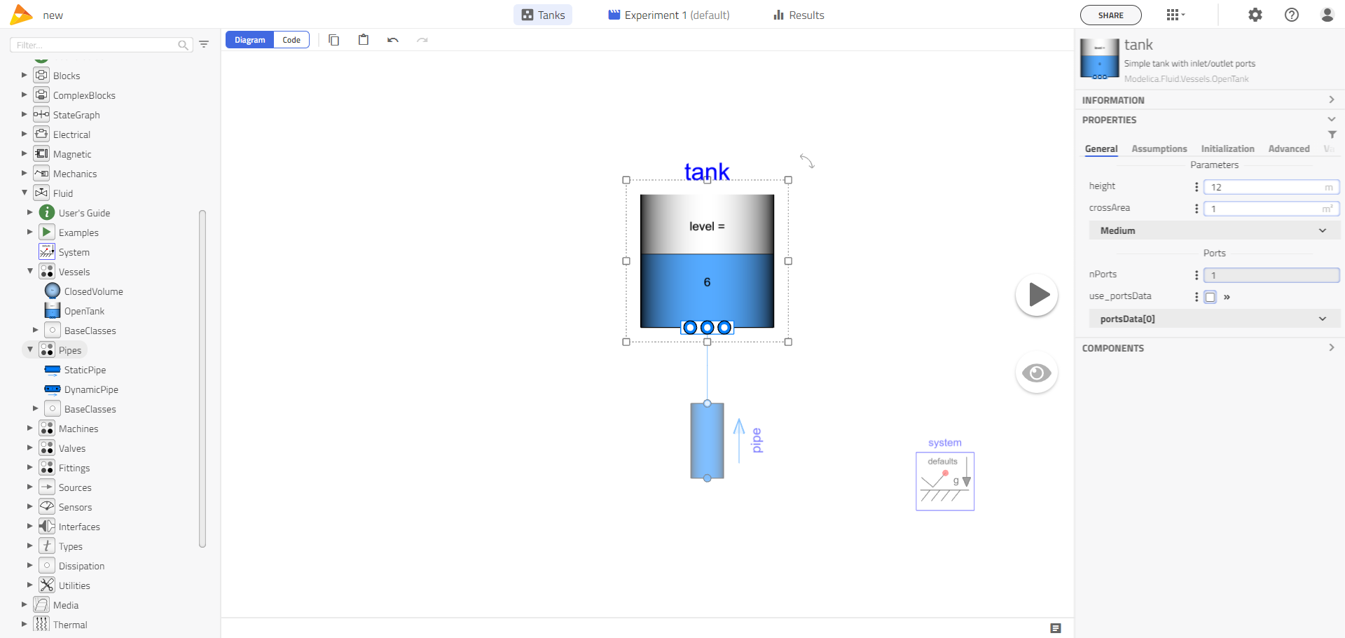
2. Select the tank component and set its properties:

   • height = 12 m (General Tab)
   • crossArea = 1 m² (General Tab)
   • use_portsData = false (Uncheck the check-box) (General Tab)
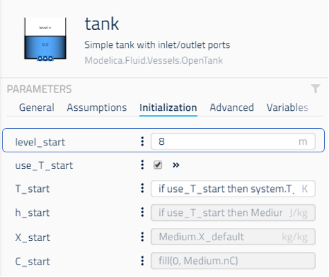
   • level_start = 8 m (Initialization Tab)

Graphic: Parameterization

There is no need to adjust other parameters, except for the setting of the media.

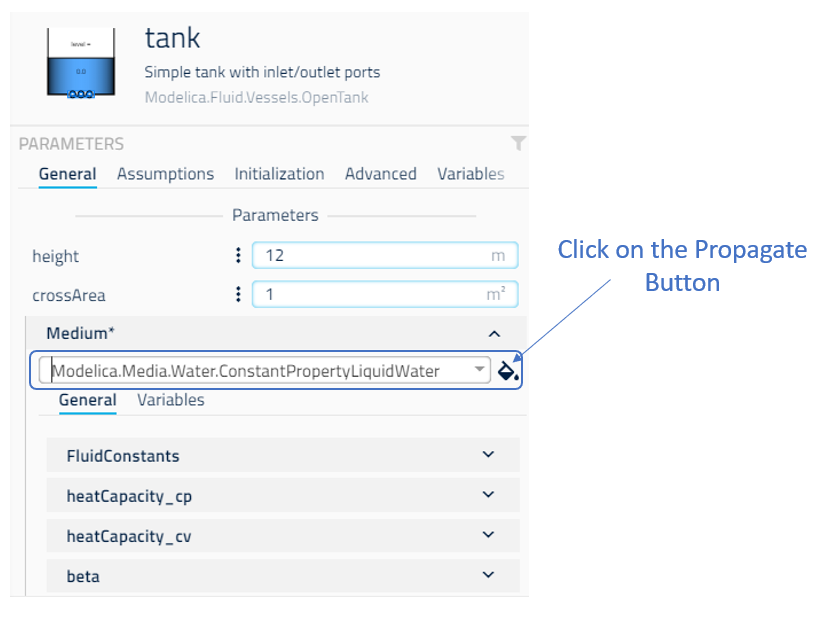
3. You will now set the media

   1. Click on Medium in the General tab.
   2. Choose Modelica.Media.Water.ConstantPropertyLiquidWater from the drop-down list and click on .

   Tip

   Type LiquidWater in the Medium drop-down list to quickly find the ConstantPropertyLiquidWater class.

Graphic: Propagation

Note

If the propagate button is missing, make sure you enable the automatic propagation in the (The link does not show proper content) settings.

4. Select pipe and set its parameters as shown below:

   • length = 2 m
   • diameter = 0.1 m
   • height_ab = 2 m

You have created the first part of the model, a tank and a pipe with their sensible properties. We will create the second part by copying the first part.

5. Select the tank and pipe components by dragging the mouse over them while holding down left-click on the canvas.
6. Copy the components given above by Right-clicking on the canvas and choose Copy.

Note

You can also use the keyboard shortcut Ctrl+C.

7. Paste the selected components by right-clicking on the canvas and choose Paste.

Note

You can also use the keyboard shortcut Ctrl+V.

8. Adjust the model layout and connect both pipes together as shown below.

   

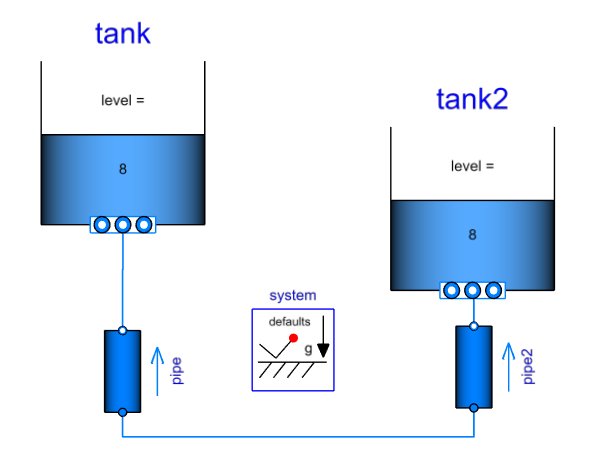
This gives us the final model layout. The remaining step is to change the initial water level within the second tank and change the tank height relative to the first one.

9. Select tank2 component and set its properties:

   • level_start = 0.01 m (Initialization Tab)

10. Select pipe2 and set its properties:

    • height_ab = -1 m

Now the model is ready for the 1^st run!

Run Simulation

You have now built the complete system model. But before you press the simulation button, you need to set up a simulation setting.

1. Switch to the Experimentation mode.

We are interested in analyzing the transient behavior (Dynamic Analysis) of the tanks.

2. Click on the Dynamic icon to activate Dynamic Analysis.

3. Set the simulation stop time to 100 seconds.

Note

Learn more about the advanced simulations settings

The experiment is now configured and you are ready to run the simulation.

4. Click the run button to start the simulation.

Note

It may take several seconds before the simulation is started as the model is first compiled.

When the simulation has finished, the result mode is activated and a new result Result1 is visible in the Results browser. The variables in Results are accessed from the Variable browser under Calculated Values.

Note

Hover the mouse over Result1 and click on three dots (...) to rename, delete, download the result file or show the simulation and compilation log.

The next step is to visualize the result!

Visualize results

Modelon Impact includes simple but powerful visualization features such as plots and stickies allowing you to inspect and analyze the result intuitively.

Results can be visualized using:

• Plots - standard way to visualize transient result
• Stickies - display variables and parameters values on the model canvas
• Built in model animation- display built-in model animation on the model canvas

Note

Result can also be exported for post-processing in other tools.

Create plots

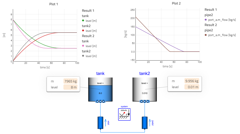
We are interested in plotting the water level in the tanks. A plot is created by dragging a variable from the variable browser into the modeling canvas.

1. Select tank1 and drag and drop fluidLevel variable on the canvas to create the Water Level plot.
2. Click on the title of the plot and rename the plot to Water Level.

Graphic: Plotting

3. Add the water level of tank2 to the same plot, by dragging and dropping tank2.Level to the Water Level plot.

4. Create a new plot (Pipe Flow) showing the mass flow through the pipe: pipe2.port_a.m_flow plot and place it next to the Water Level plot.

   

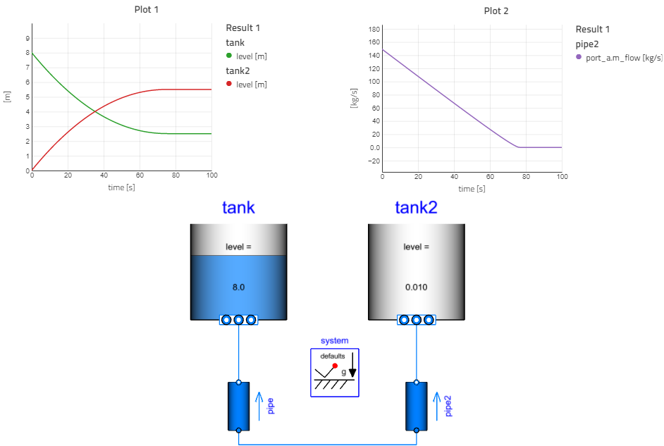
Analysis: Initially water is flowing from the tank with the higher water level to the lower tank. The water levels in both tanks will stabilize around an equilibrium point when the static pressure from the tanks including the pipe height is equal on both sides.

How can I change units?

Tip

Each plot can be exported to a .png image or .csv file.

X-Y Plots

It is also possible to create parametric plots where the independent variable is not 'time.' We will now create a plot for the level of fluid in tank2 as a function of the level of fluid in tank1.

1. Create a new plot by dragging and dropping the variable tank2.level onto an empty portion of the canvas.
2. Click on the title of the plot and rename it to Water Level (Parametric).
3. Now drag the variable tank1.level onto the x-axis of the plot to make it the x-variable.

Graphic: X-Y Plot

A new plot is created if the variable is dragged to an empty space in the canvas. If dragged onto an existing plot the variable is added to the same plot. If dragged onto the x-axis of an existing plot, the selected variable is chosen as the independent variable; this will generate a parametric x-y plot. It’s also possible to drag variables between plots.

The Time Slider at the bottom of the canvas can also be used to show a line marker in each plot with time on the x-axis.

Built-in animation

The tank model has built-in diagram animation that is useful for quickly getting an overview of the system. A time slider will automatically appear on the modeling canvas after simulation.

1. Slide the time slider and check the model behavior from 0 sec to 100 sec. It is also possible to use keyboard arrows to move through time up and down.

   

Stickies

The sticky represents a label connected to a specific component or model.

There are 2 types of stickies:

• Not Editable (Result Variables)
• Editable (Inputs)

Non-editable sticky can be created by clicking on the icon next to each variable.

1. Enable stickies for,

   • tank.m
   • tank.Level
   • tank2.m
   • tank.Level

Graphic: Stickies - Non-editable

Tip

Moving the time slider will update the values in the stickies.

An Editable sticky can be created by hovering over the required variable and click on the icon.

1. Create an editable sticky for pipe.General.Geometry.diameter.

Graphic: Stickies - Editable

Views

We have just prepared a good view example including 2 plots and several stickies. This view can be saved by hovering the mouse cursor over the run button and saving it.

1. Create a new view called Basic View. Refer to Views for more detailed information.

Result Comparison

It is possible to re-run the model with the adjusted pipe diameter and compare the results with the 1^st run.

1. Change the diameter = 0.2 m in a pipe and press the Run button.

Graphic: Compare Results

Increasing one of the pipe diameter allowed reaching the same water level faster as expected.

Congratulations, you have modeled, simulated and analyzed your 1^st model!