Experiment 1: Orifice Sizing
The first experiment is devised to solve the orifice sizing problem, deriving a suitable orifice diameter for each branch based on a design mass flow.
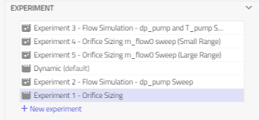
1. Navigate to the experiment tab at the top panel:
2. Select the experiment "Experiment 1 - Orifice Sizing"
When in the experiment tab, you can see which modifications have been made to the model for the purpose of the experiment definition as below:
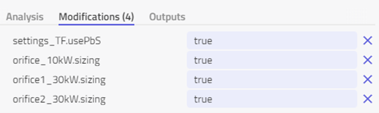
In this case, the flag usePbS is set to true to enable Physics-based Solving. For each of the three orifice components, sizing is also set to true which correlates to the sizing being determined based on the design mass flow rate m_flow0.
Assumption: For the problem outlined, it is assumed that a design factor of 30kW/kg/s is in place for the coolant. In other words, a flow rate of 1 kg/s will be able to evacuate a heat load of 30kW. By summing the total heat loads in each of the three branches, the corresponding m_flow0 values will be assigned for the respective orifices. For example, the right-most orifice orifice2_30kW needs to evacuate the combined heat loads from the eMotor (20kW) and inverter2 (10kW) making up 30kW. The design flow rate m_flow0 is thus set to (30/30) kg/s = 1 kg/s.
Results
To interpret the results of this first experiment, the following steps should be carried out
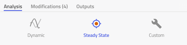
1. Select Steady State under the Analysis tab for the experiment:
2. Simulate the experiment Experiment 1 - Orifice Sizing.
3. Select the results tab and name the result with the same name as the experiment.
4. Under system views, enable "Experiment 1 - Sizing, Pressures and Flows"
The result should look as follows:
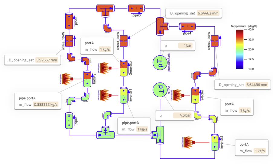
Figure 2: Results from orifice sizing experiment - Orifice sizes, pressures and mass flow rates.
The components are color-coded to visualize the temperature distribution in the branches. The coolant is heated up as it flows through the EPS components. As depicted in the color bar, the fluid temperature does not exceed 40°C at any point in the circuit, hence all components are adequately cooled based on the set max temperature requirements.
- The calculated orifice diameters from the flow balancing problem are indicated with stickies denoted as D_opening_set. The corresponding flow rates in each branch are also displayed as m_flow0 at selected fluid ports.
- The middle and right orifice branches both need to evacuate a total heat load of 30kW, hence they have resulted in the same orifice sizing of approx. 6.64mm, however, the left orifice branch only needs to evacuate 10 kW of heat from the battery, hence a smaller diameter of approx. 3.93 mm was calculated.
A more precise reading of the inlet and outlet temperatures at each electric component in the fluid circuit can be visualized by enabling the system view Experiment 1 - Temperatures:
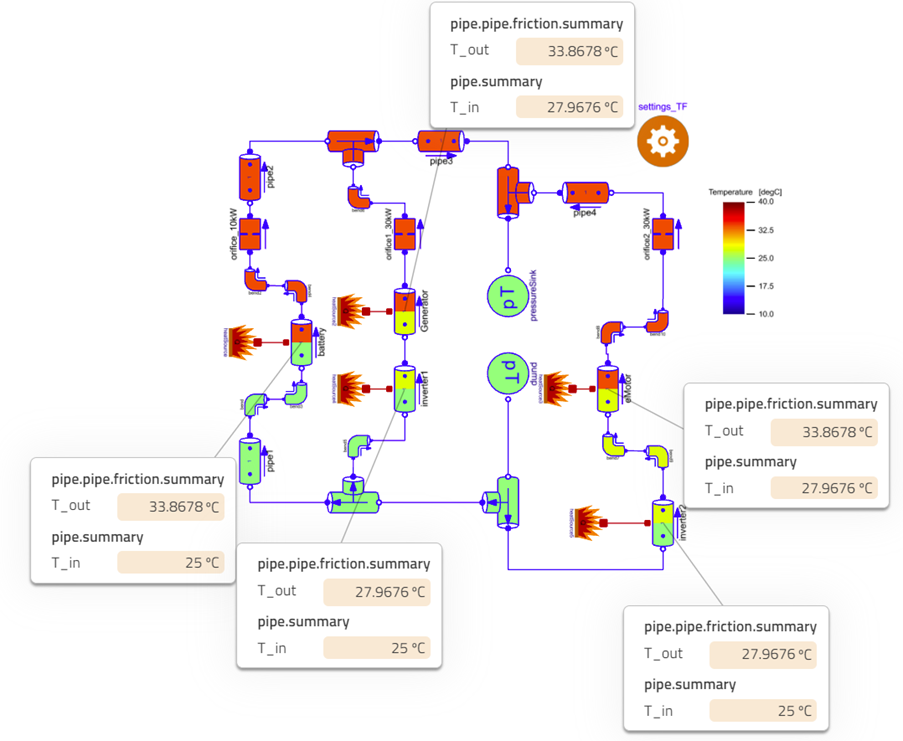
Figure 3: Results from orifice sizing experiment - temperatures at select points.
Bonus Exercise:Building Experiment 1 from scratch
The predefined experiments in this model are read-only, hence cannot be modified or duplicated. If interested in building an editable experiment of any of those included in the model, the user can do so by creating a new experiment. The steps below outline how to create a new experiment identical to Experiment 1 outlined above.
1. Create a new experiment in the experiment tab and name it appropriately.
2, With the newly created experiment created, click on the settings_TF cog icon and enable the flag usePbS
3. Select components "orifice_10kW", "orifice1_30kW" and "orifice2_30kW" one by one and enable the parameter sizing in each.
4. Note the newly added modifications appearing in the experiment view as a result of the changes made in steps 2 and 3.
5. Ensure steady-state is selected under the analysis tab and simulate.
The results obtained should match those from the predefined experiment 1.
Further modifications can be made to this experiment for any additional analysis as well as creation of duplicate experiments by right-clicking on this one and selecting "Duplicate". Experiments can also be deleted by right-clicking and selecting "Delete". Note that that the default experiment cannot be deleted, however, the default experiment itself can be changed by right-clicking and selecting "Set as Default",