Base

This experiment illustrates how the VaporCycle.Experiments.HeatPump model can be easily configured to run a steady-state simulation with the Physics-based Solving capability of Modelon Impact. The model has already been parameterized with the appropriate modifications needed to executed with the steady-state solver, given that variability_propagation has been enabled in the steady-state compiler settings.

In the Experiment section below, a workflow is outlined to demonstrate how one system model can be used for both dynamic and steady-state to reach the same equilibrium results. The first time is with the dynamic solver to see the transients imposed like the original example. The second and third time will be with the steady-state solver to match the equilibrium operating conditions before and after the transient period.

Note: This model will not simulate as-is with dynamic simulation unless settings_TF.usePbS is set to false.

Parameterization

This model extends from VaporCycle.Experiments.HeatPump and modifies components in order to enable PbS functionality and propagate start values. Good and consistent initialization throughout the system will lead to a better rate of convergence when using steady state execution. The following modifiers have been made:

settings_TF

By setting usePbS = true, component models that support PbS will enable the PbS annotations to be used with the steady-state solver

liquid sink boundaries

For PbS, sources and sinks must be identified using the parameter isSource. By default, this is true so the sinks must be updated

liqOut_Evap.isSource = false
liqOut_Cond.isSource = false

compressor

fixedPressure = true. For the closed-loop system the pressure needs to be grounded somehow. In this case the high side pressure will be fixed.
isP_suc = false. If true, the suction pressure is fixed, else the discharge pressure is. For this example, the discharge pressure will be fixed via init.p_high
p0_dis = init.p_high. Propagating the initialization for the discharge pressure from the init record.
p0_suc = init.p_suction. Propagating the initialization for the suction pressure from the init record.
m_flow_start = init.mflow_start. Propagating the initialization for the mass flow rate from the init record.
dp_start = init.p_high - init.p_suction. Propagating the initialization for the pressure differential from the init record.
Initial values are set and propagated from the init record for better convergence and ease of system parameterization from one location.

expansionValve

SuperHeatSetPoint = init.T_sh. Propagating the superheat set point from the value set in the init record so that all system initialization would be based on the same expected superheat.
dp_start = init.p_high - init.p_suction. Propagating the initialization for the pressure differential from the init record.

superHeatSensor and subCoolingSensor

allowNegative = true. When superheat or subcool is being controlled, having negative values allowed removes a singularity when the refrigerant is in the two-phase region.

Experiment

Switch to the Experiment mode (or press [2] on the keyboard) and create a new experiment named Dynamic
With the Dynamic experiment selected, disable settings_TF.usePbS so it is false. Then confirm that the change is listed under Modifications for the Dynamic experiment
Make sure the Analysis mode is changed to Dynamic with a Stop Time of 800s and run the experiment.
Rename the result as Dyn and plot the variables listed below. Then create a View with them called Plots.

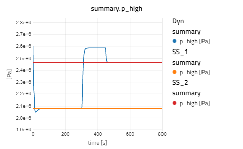
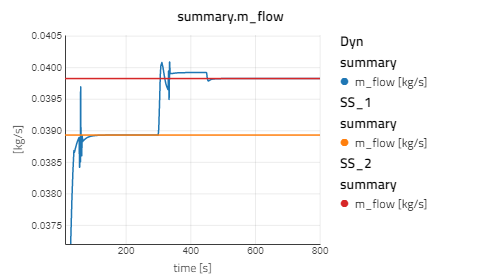
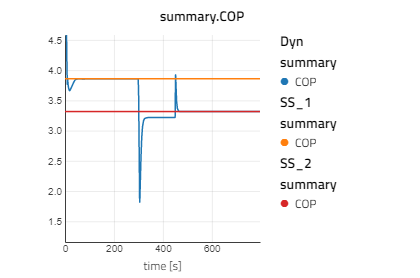
liqIn_cond.m_flow_in, the liquid mass flow rate into the condenser
liqIn_cond.T_in, the temperature of the liquid into the condenser
summary.p_high, the high side pressure discharged from the compressor as fixed for steady-state
summary.m_flow, mass flow rate of the refrigerant
summary.COP, coefficient of power as the heat flow rate from the condenser divided by the provided compressor power

Note that there are transients imposed on the liquid source into the condenser from the ramp blocks, and that there is a period of equilibrium before (time = 200 s) and after (time = 600 s).
Next will be the steady-state simulation. In Settings > Execution > Steady State > Compiler Options turn on variability_propagation. Also make sure 'Enable steady state simulation' is enabled in the Settings > Application
Switch to the Experiment mode and create a new experiment named SteadyState_1
Based on the dynamic result, the high side pressure before the transients is 2077100 Pa. Set init.p_high = 2077100 so that the high side pressure is fixed to the new value and propagated for initialization. Confirm that it is listed under Modifications.
Make sure the Analysis mode for SteadyState_1 is set as Steady State and run.
Rename the result SS_1 and check the plots using the Plots View. The steady-state result should overlap with the first equilibrium period of the dynamic result.
Switch to the Experiment mode and create one last experiment named SteadyState_2
In order to match the second equilibrium operating condition, the high side pressure and also the conditions of the liquid flow into the condenser need to be updated. The high side pressure can be determined from the dynamic result and the liquid conditions are already known from the ramp source blocks connected to the liqIn_cond boundary.

init.p_high = 2464800 Pa
init.mflow_cond_sec = 0.3 kg/s, this will be set as the offet in mflow_cond
init.T_cond_sec = 321.15 K, this will be set as the offset in T_cond

Confirm that the changes are listed under SteadyState_2's Modifications.
Make sure the Analysis mode for SteadyState_2 is set as Steady State and run.
Rename the result SS_2 and check the plots to see that the new results overlap with the second equilibrium period of the dynamic result.

Results

The plots below have been zoomed-in.