PID Autotuner🔗
Introduction🔗
A proportional-integral-derivative controller (PID controller) is a widely employed, understandable and effective component to continuously control a system, subsystem or single component. It applies a correction based on the difference between a desired setpoint and a measured process variable. To calculate the controller output, three control terms are used: proportional, integral and derivative terms. A user needs to provide three corresponding PID parameters, typically the gain kp of the controller, the time constant of integrator block Ti, and the time constant of derivative block Td. Since every system has unique properties in terms of responsiveness, finding the right parameters can be challenging. There are several different rule-based tuning methods, typically involving an artificial change to the controlled component and then observing the system response to derive appropriate parameters. One of these rule-based methods is AMIGO Tuning.
The Modelon Base Library includes a model that uses the AMIGO tuning method to find appropriate values for the proportional gain k, integral time constant Ti, and derivative time constant Td.
Purpose of the tutorial is to show how to use Modelon's PID Autotuner model to find the PID parameters of a controlled system.
About the tutorial🔗
Time to complete this tutorial is approximately 20-30 minutes.
The system for which we want to get the PID parameters is a model that controls the CO2-level in a room involving a changing number of people. Fresh air is blown into the room depending on the trace volume of CO2. The inflow of CO2 depends on the number of people in the room. Accordingly, our PID model uses the trace volume of CO2 as a measured process variable and outputs the mass flow of fresh air to adjust the CO2-level to the desired setpoint.
The tutorial shows how to integrate the Autotuner model in the example model RoomCO2WithControls from the Modelica Standard Library, and how to configure the model to obtain PID parameters.
You will learn how to:
- Integrate the Autotuner into an existing model
- Set Autotuner parameters according to system properties
- Create views to get some understanding of the Autotuner model
- Obtain PID parameters
- Compare the obtained PID parameters for different Autotuner settings.
Preparation🔗
The Autotuner example model requires to have Modelon Impact Pro version license, which includes all Modelon libraries.
The ![]() Modelon Base Library will be used in this workshop.
Modelon Base Library will be used in this workshop.
The instructions are valid for Modelon Impact on cloud.
-
Run Modelon Impact.
-
Create a new workspace called PID_Autotuning
We are now ready to start building the model!
Tip
In this tutorial we will only build one model with the PID Autotuner to control the CO2-level in a room. If you want to try another model by yourself (see the end of the tutorial), we recommend to create a package structure for each example. This way we can keep our workspace organized.
Build model🔗
We will build the model using the existing example model RoomCO2WithControls from the Modelica Standard Library.
-
Navigate to
Modelica.Fluid.Examples.TraceSubstances.RoomCO2WithControlsand duplicate the model to your workspace. -
Rename your new model to "RoomCO2WithControls_PID". This is our reference model with the standard PID component.
-
Duplicate the model again and name the new duplicate "RoomCO2WithControls_Auto". This is the model that we will use to tune the PID parameters.
-
Open "RoomCO2WithControls_Auto" and delete the PID component.
-
Navigate to
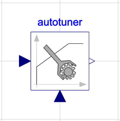
Modelon.Blocks.Control.Autotunerand drag the component onto the model canvas. Place it in betweenCO2Setandgain1. -
Connect
CO2Setto the left input of the Autotuner, connectgainSensorto the bottom input of the Autotuner, and connect the Autotuner output togain1.
Your model should now look like this:
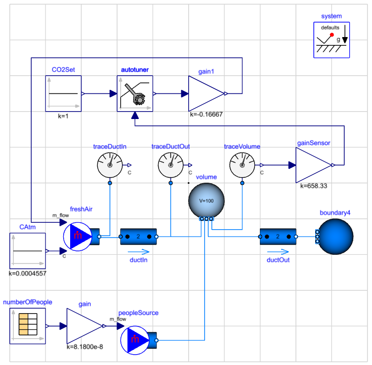
We are now ready to set the component properties.
Parameterization🔗
General🔗
To parameterize the Autotuner, we need to have a basic understanding of our controlled system. So let us look at some parameters of the Autotuner and how we can derive reasonable values from the system model.
Limits of PID output signal
We are directly controlling the mass flow of the fresh air. The maximum mass flow of fresh air is limited to 1/6 kg/s. There is a gain model that multiplies the PID/Autotuner output signal by a constant factor of -1/6. This means we need to limit our Autotuner output signal to values within the range of 0 and -1.
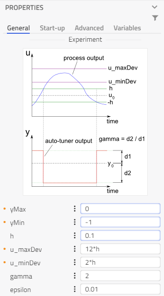
In the General tab of the Autotuner model, set yMax to 0 and yMin to -1.
Deviation of measured PID input signal
The process output, or PID/Autotuner input signal, is in our case the CO2 trace volume. We want to parameterize the PID controller in a way that the CO2 concentration does not exceed 1000PPM (=1.519E-3 kg/kg). At the same time, we want to keep the mass flow of fresh air as low as possible to save energy.
Using a fixed setpoint while not allowing any deviation from it likely leads to the chattering of the PID controller. The controller will be stuck in re-adjusting its output signal. To overcome this issue, a hysteresis band is used. Instead of a single setpoint value u0, we define a band with the bounds [u0+h, u0-h], with h as the hysteresis level. When the process output signal crosses both bounds, the PID controller starts/stops adjusting its output signal.
In the Autotuner model, the hysteresis level h can be set. Furthermore, there are two more parameters that can be set to define the target maximum and minimum deviation of the process output, u_maxDev and u_minDev. The Autotuner model can not find a solution, if u_maxDev is smaller than the hysteresis level h. So it is advisable to set the deviation limits in relation to the hysteresis. Let us start with a ballpark hysteresis level:
-
In the
Generaltab of the Autotuner model, sethto 0.1 -
Use the default values for
u_maxDevandu_minDev.
Your General tab should now look like this:
Start-up🔗
The Autotuner will induce changes to the fresh air mass flow and then analyze changes in the CO2 trace volume. It will only work if the system transients are negligible, i.e. it is in steady-state or near steady-state. Otherwise, strong system transients will overlap with the induced changes and the Autotuner model derives faulty PID parameters. This means that we need to remove all changing boundary conditions. In our case, the only changing boundary condition is the number of people.
-
Remove changing boundary conditions.
-
Delete the component
numberOfPeople. -
Navigate to
Modelica.Blocks.Sources.Constant, drag the component onto the canvas and connect it to thegaincomponent. -
Set the constant value
kto 10.
-
The next step is to set the start-up parameters of the Autotuner model.
The Autotuner model starts tuning after the (near-)steady state has been reached. In the Start-up panel of the model, there are several parameters that can be used to tell the Autotuner how and when steady-state is reached.
The useController option can be used for unstable systems that require controlling to reach a steady state or in some cases to shorten the time required to reach the steady state. If enabled, a PI controller will determine the output of the Autotuner model. Correspondingly, you need to provide PI parameters that can be used to reach a steady state. If disabled, the Autotuner will have a constant output. This can be used if the system quickly reaches a steady state with a constant system input. In our case, the system reaches a steady state with a constant system input. However, we want to speed up the process, so we use the PI controller option.
In the Start-up tab of the autotuner block,
-
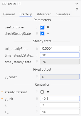
Enable
useController. -
Set
y_initto -0.1. Keep the default values fork(=2) andT_i(=50).Note
Make sure to initialize your system with a mass flow that is greater than 0. Setting it to zero most likely leads to failure in the tuning process.
There are two ways to tell the Autotuner model that a steady state has been reached. The first method is by defining a time after which a steady state in the system has been reached. This can be used for systems, where we know the behavior beforehand and after what time it reaches a steady state. This option can be toggled by disabling the checkSteadyState option. The second method is to use the built-in check function for the steady state. In that case, we need to provide a tolerance and a starting time for the check function to become active. This option can be toggled by enabling the checkSteadyState option. Let us use the second option for our model.
-
Enable
checkSteadyState. -
Use the default values
tol_steadyState(=0.0001) andtime_steadyStateCheck(=10).
Your Start-up tab should now look like this:
We are now ready to run our model!
Run Simulation🔗
We have now built the complete system model. But before we press the simulation button, let us look at the simulation setting.
- Switch to the Experimentation mode.

- Check that the following experiment parameters are set correctly:
- Execution mode is set to Dynamic.
- Start Time is set to 0 s, Stop Time is set to 86400 s.
- Under the Advanced settings, Tolerance is set 1e-8.
Note
The Autotuner model stops the simulation as soon as it has found the PID parameters. If it cannot find PID parameters, the simulation will run until the defined Stop Time. It is advisable to set the Stop Time to a high value to not stop the Autotuner model prematurely.
The experiment is now configured, and you are ready to run the simulation.
- Click the
 run button to start the simulation.
Note
It may take several seconds before the simulation is started as the model is first compiled.
When the simulation has finished, the result mode is activated and a new result Result1 is visible in the Results browser. The variables in Results are accessed from the Variable browser under Calculated Values.
- Rename the result to Undertuned
The next step is to visualize the result!
Visualize results🔗
To get a brief understanding of what the Autotuner does, let us first look at the input and output of the Autotuner model.
Tip
Click here to learn how to create plots.
- Select autotuner and plot the variable
u_m.
Tip
Click the input connector of autotuner to immediately filter your calculated values to just u_m.
- Create another plot showing the autotuner output: autotuner.y plot and place it below the previous plot.
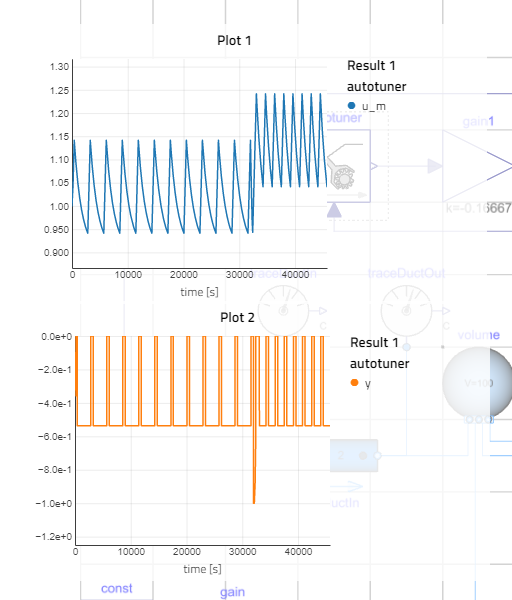
We can see how the Autotuner periodically alternates the output signal and analyzes the system response. After a few periods, the output signal is changed to a different, periodic alternation. The system response is again analyzed and the autotuner model stops the simulation after some time.
Close the two plots as we do not need them anymore.
Next up, let us look at how to get the calculated PID parameters out of the model. In Modelon Impact, we can use stickies to show a single value in our model.
A sticky can be created by clicking on the ![]() icon next to each variable.
icon next to each variable.
-
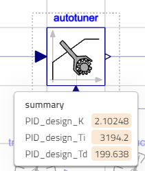
Enable stickies for,
- autotuner.summary.PID_design_K
- autotuner.summary.PID_design_Ti
- autotuner.summary.PID_design_Td
The Autotuner updates these values at the last time step. To get the values we need to set the time to the end.
- Use the time slider at the bottom to change the time to the stop time.
You can see the PID parameters update at the stop time.
- Create a new view called PID parameters, so we can quickly get the parameters in future runs.
We are now ready to test our parameterization with the actual PID model.
Evaluation🔗
To see if our newly found PID parameters are useful for our original controlled system, we can put them into the original PID model-controlled model. But first, let us run the PID controlled system with the default values. The results of this run will serve as a comparison.
-
Create the Default case.
-
Go into "RoomCO2WithControls_PID", the model that we created at the beginning.
-
Have a look at the default values for
k,Ti, andTdin the PID model.
Note
The default setup uses a PI controller. Therefore,
Tdis deactivated.-
Set
yMaxto 0 andyMinto -1. -
Run the simulation.
-
Rename the result to Default.
-
Plot the PID input signal
PID.u_m.
-
In a well-tuned controlled system, the input signal should not exceed 1 (corresponding to 1000PPM) and the system should be stable. As we can see, the results are below 1 most of the time. However, there are some spikes temporarily pushing the CO2 level above 1000 PPM, and also indicating some instability in the controlled system.
Let us have a look at how our newly found PID parameterization performs.
-
Compare to the first Autotuner parameterization.
-
Go back to the modeling screen and change the
controllerTypeto PID. -
Copy the values for
k,Ti, andTdfrom the Autotuner model to the PID model.
You can right-click the value of our sticky and select Copy value to quickly transfer the values to the corresponding PID parameter field.
- Run the simulation. Rename the result to Undertuned
-
If your plot for the PID input signal is still open, it will automatically update the plot to include our latest result. Otherwise, create a new plot where you drag in PID.u_m for the Default and the Undertuned case. We can see that our Undertuned solution does not work well to limit the CO2 level below 1.
Let us try to find a better solution.
-
Go back to the modeling view of
RoomCO2WithControls_Autoand setautotuner.hto 0.001. -
Run the simulation. After it has finished, name the result as Tuned.
-
Go back to the modeling view and set
autotuner.hto 0.00001. -
Run the simulation. After it has finished, name the result as Overtuned.
Let us go back to our PID model to test the two new parameter sets.
- Repeat step 2.2 and 2.3 with the Tuned parameter set and the Overtuned parameter set.
Note
The Overtuned case does not finish, as the solver is unable to simulate with a parameterization that is too strict. We can abort this simulation after some time.
We now have our four cases (Default, Undertuned, Tuned, Overtuned) in our plot. To further analyze the latest results, delete the Undertuned case. As we can see, our Overtuned solution does not finish and we can not use it here. However, our Tuned solution shows good results without spikes above 1, while finishing the simulation in a reasonable amount of time.
Congratulations, you have learned how to use our PID autotuner model!
If you want to try to find PID parameters for another model, you can have a go at VaporCycle.Experiments.AirConditioning. Remember to deactivate all changing boundary conditions here.