Build Turbojet model
Introduction🔗
A jet engine is a type of reaction engine discharging a fast-moving jet that generates thrust by jet propulsion. It is well known, especially from the various types of aircraft. The definition is quite broad since it can include rockets, water jets, and hybrid propulsion. The term jet engine typically refers to an air-breathing jet engine such as a turbojet, turbofan, ramjet, or pulse jet. In general, jet engines are combustion engines.
![]()
Modelon Jet Propulsion Library provides a foundation for the modeling and simulation of jet engines, including the model-based design of integrated aircraft systems. It can be connected directly to other Modelon libraries that are part of Modelon Impact Pro.
Tip
Jet Propulsion Library can use both dynamic and steady-state solvers. The steady-state solution naturally supports Physics Based Solving technology, allowing efficient computation of the steady-state solution.
Before we start🔗
You will need approximately 60 minutes to finish all tutorial steps.
What are we building?
This application is designed as a workshop, where we'll show how to build a simple turbojet model consisting of all essential parts. The resulting model will roughly resemble the famous GE J85 from the 1950s.
You will learn how to:
- Prepare and set up all essential parts
- Build a simple turbojet
- Run it in different conditions using steady state solution
Preparation🔗
The turbojet model requires to have Modelon Impact Pro version installed, which includes all Modelon libraries.
Two libraries: ![]() Jet Propulsion and
Jet Propulsion and
![]() Electrification libraries will be used in this workshop.
Electrification libraries will be used in this workshop.
Enable custom functions🔗
Jet Propulsion is shipped with custom functions used for the steady-state solution.
We need to make these custom functions available in Modelon Impact. Those functions are placed within the Resources folder.
Custom functions will be automatically loaded once the libraries are drag and dropped to GUI.
-
Copy files from Modelon Impact installation (e.g.
<modelon_impact_installation_folder>/modelica-dist/JetPropulsion X.X/Resources/custom_functions) toC:/Users/<user_name>/impact/custom_functions. Create the foldercustom_functionsif it does not exist. -
Copy files from Library Resources (e.g.
impact/workspaces/<workspace_name>/model_libraries/<editable or read_only>/JetPropulsion X.X/Resources/custom_functions/) toimpact/custom_functions/.
- Run Modelon Impact.
Note
If Modelon Impact is run before copying the files, they will not be available. The order is important.
-
Create a new workspace called turbojet.
-
Create a new model called turbojet.
-
Hover your mouse over the play button and you should see custom functions available.
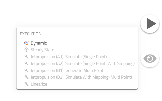
If the custom functions are not visible, go through the steps again checking for spelling and re-launching Modelon Impact.
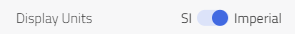
Default units selection🔗
In this tutorial, we use imperial units since they are common references on the chosen engine.
-
Go to the settings
 .
. -
Within the Units tab, change SI units to Imperial.
- Save and close the Options window.
We are ready to start building the model now!
Simple model🔗
The model that will be built resembles the GE J85. The model will be steady-state, including one design point.
Geometry🔗
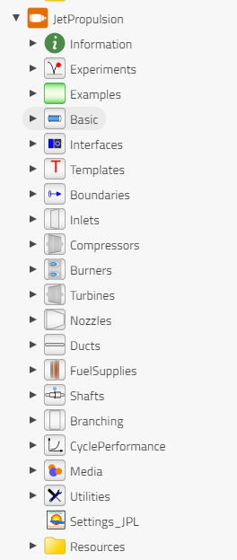
We will build the model on a single level and primarily use components from JetPropulsion.Basic.
Note
It is essential to use components from the Basic sub-library in the JetPropulsion library.
-
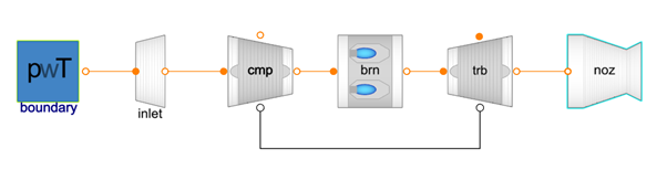
Identify the components in the model diagram, find them in the JPL library and add the components to the turbojet model canvas:
JetPropulsion.Basic.Inlets.Inlet
JetPropulsion.Basic.Compressors.Compressor
JetPropulsion.Basic.Burners.WithInputPort
JetPropulsion.Basic.Turbines.Turbine
JetPropulsion.Basic.Nozzles.Nozzle
JetPropulsion.Boundaries.AmbientBoundary
JetPropulsion.Settings_JPL
Modelon.Environment.AirDataImplementations.XYZ
Modelon.Environment.AtmosphereImplementations.US76
Modelon.Environment.WorldRepresentation
Note
The component names you find may not match up with the tutorial as they have been changed for clarification. You can change their name to match the tutorial by opening the right-hand menu, clicking on the component and editing the name in the top right corner next to the component icon.
- Connect components in series as shown below.
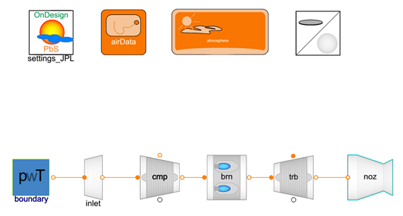
- Connect the compressor and turbine with the black mechanical connection line, representing a shaft.
Note
This is an ideal mechanical connection without losses or inertia.
Model parameters🔗
We will parameterize the model using information about the GE J85 on Wikipedia (and a few additional sources mentioned at the end of this tutorial).
The performance data on the engine are shown below:
| Performance | |
|---|---|
| Maximum thrust | 2,850 lbf (12.7 kN) (dry) |
| Overall pressure ratio | 7 |
| Air mass flow | 158400 lbm/h (20 kg/s) |
| Turbine inlet temperature | 1,640 °F (893 °C) |
| Specific fuel consumption | 0.99 lbm/(lbf.h) or 27 g/(kN.s) |
| Shaft speed | 16500 rpm |
All data refer to sea-level static conditions.
 Boundary🔗
The boundary model prescribes the total pressure and temperature using ![]() the Atmosphere component.
Prescribe the mass flow rate at the boundary element by setting w=158400 lbm/h (20kg/s) in the General tab.
the Atmosphere component.
Prescribe the mass flow rate at the boundary element by setting w=158400 lbm/h (20kg/s) in the General tab.

 Inlet🔗
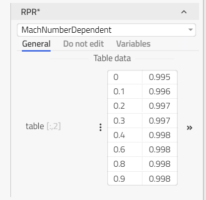
A ram pressure recovery presents the main parameter of this component.
-
Expand the RPR (Ram Pressure Recovery) group.
-
Choose the Mach number dependent RPR:
JetPropulsion.Basic.inlets.RamPressureRecovery.MachNumberDepententand keep the default setting.
 Compressor🔗
-
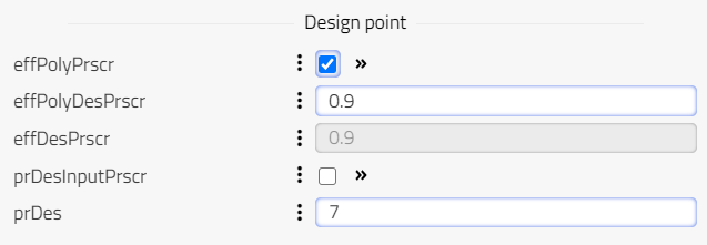
Set the design pressure ratio prDes to 7.
-
Enable effPolyPrscr to prescribe compressor design point efficiency in terms of polytropic efficiency. Set the design polytropic efficiency effPolyDesPrscr to 0.90, i.e., 90%.
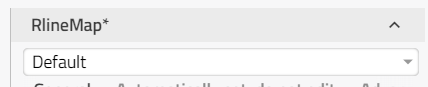
- Select
JetPropulsion.Basic.Compressors.RlineMaps.Defaultfrom the drop-down menu in RlineMap. It is an R-line map using replaceable tables in imperial units (without visualization).
- Next, inside the RlineMap open the Table group and from the drop-down select JT9D High Pressure Compressor map:
JetPropulsion.Compressors.Sections.Examples.JT9D.Components.Maps.HighPressure.
Note
This pressure ratio and the efficiency define how much (mass flow rate specific) power the compressor requires for the on-design computation (together with the mass flow rate we can compute the dimensional power).
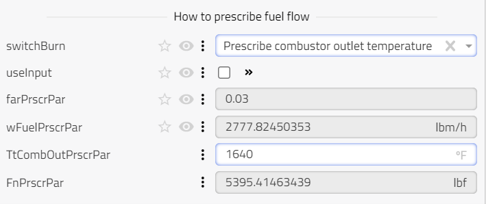
 Burner🔗
-
As we want to prescribe outlet temperature, change switchBurn to the prescribed temperature:
JetPropulsion.Basic.Burners.Internals.SwitchBurn.Temperature -
Set the temperature parameter TtCombOutPrscrPar to 1640 °F (or 2100 R, 893 °C, 1166 K)
Note
If you want to create a more accurate model then additionally select the constant value function for the burner efficiency, and enter a value of 0.98, also, enter a duct pressure loss dpqpf of 0.05. This yields a slightly more realistic real burner efficiency and includes some wall friction.
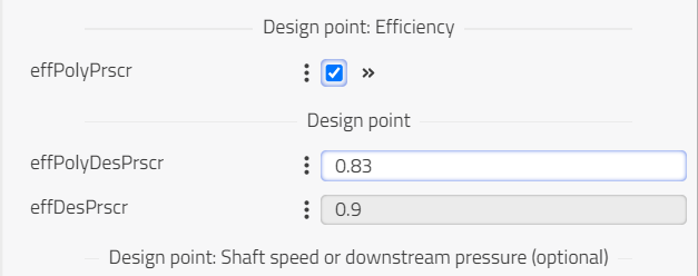
 Turbine🔗
-
Set the (uncorrected) design shaft speed NDesPrscr to 16500 rpm.
-
Set the design polytropic efficiency effPolyDesPrscr to 0.83, i.e., 83%. Again, remember to enable effPolyPrscr.
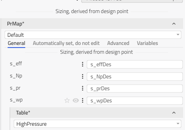
-
Make sure the
JetPropulsion.Basic.Turbines.PRmaps.Defaultis selected within the PrMap. It is the default pressure ratio map using replaceable tables in imperial units (without visualization). -
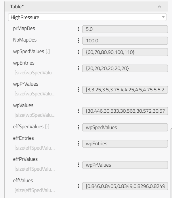
Expand the Table drop-down and select JT9D High-Pressure Turbine (HPT) map:
JetPropulsion.Turbines.Sections.Examples.JT9D.Components.Maps.HighPressure.
 Nozzle🔗
For the nozzle, no parameters have to be touched to yield a working model.
Note
If you want to create a more accurate model, expand the friction group and select the constant value option. Enter dpqpPrscr of 0.1. This will include wall friction for the nozzle. Additionally, deselect useCV to use the gross thrust type nozzle performance correlations (instead of the velocity coefficient). In the group corresponding to the converging-diverging nozzle chosen by default (ConDivThrustCoefficient), select a constant value option, too. Enter a value of 0.98 for CFgPrscr.
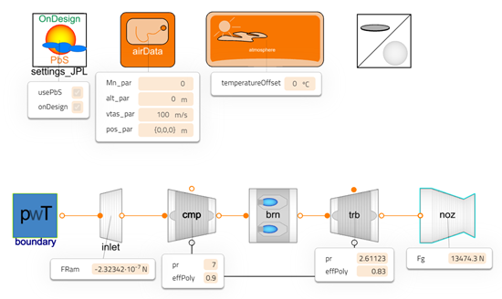
 Ambient conditions🔗
In this example, we will use a simple setup of the boundary conditions. We will only change altitude and Mach Number. We will only work with the standard day conditions (and will not impose any temperature offset). Change your model such that you simulate sea-level static conditions as follows.
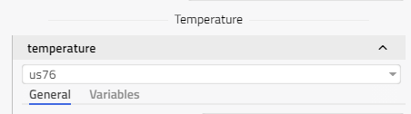
- Make sure the standard day
Modelon.Environment.Utilities.Functions.Temperatures.us76is used in the atmosphere model.
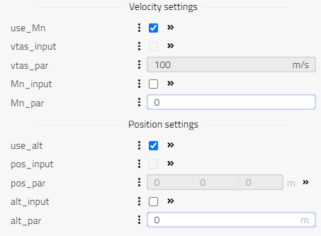
- In airData model, set the Mach Number Mn_par to ‘0’ and the altitude alt_par to ‘0’ ft.
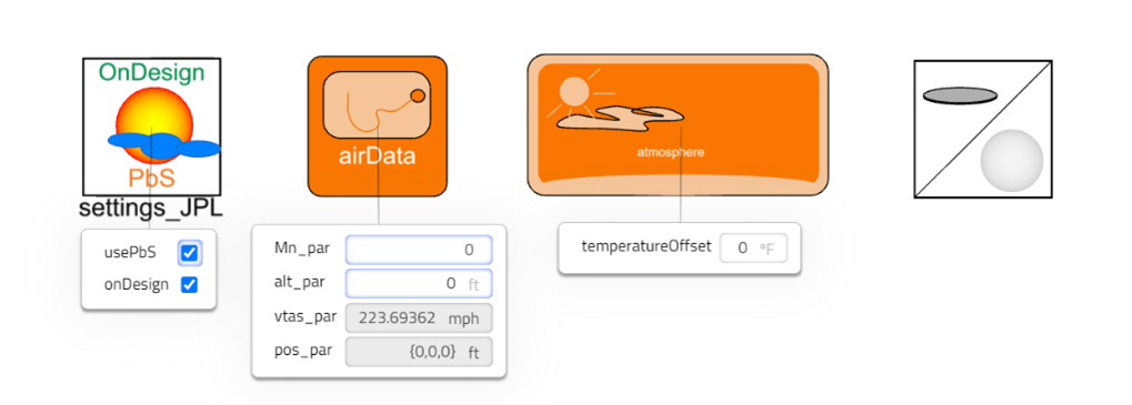
- Switch on the case setup view to see the following parameters of the ambient conditions on the canvas: alt_Par, Mn_Par, temperatureOffset, usePbS and onDesign.
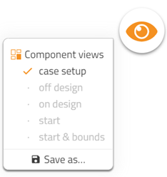
The sticky window will appear next to the Environment Models.
Tip
Sticky is added by clicking on the eye symbol next to a variable. Click here to learn how to create additional stickies.
- Check the box next to usePbS in settings_JPL as shown below.
Note
onDesign is a global switch for running model on-design (to compute component sizing) vs. off-design (to compute off-design performance given some component sizing). See library help for more details (JetPropulsion, Information, User's Guide, Technical Notes, Simulation Modes).
PbS stands for the steady-state "Physics based Solving".
Running the model🔗
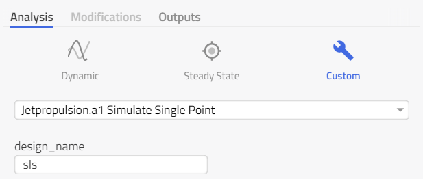
- Go to the Experimentation mode (click on it).

- Select Jetpropulsion (A1): Simulate (Single Point) custom function by hovering your mouse over the run button.
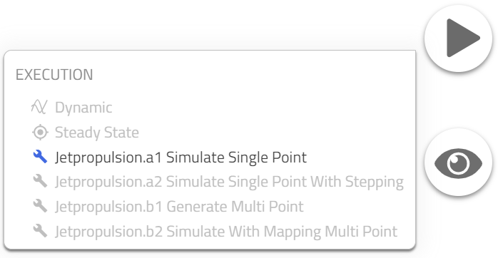
-
Adjust the design_name to sls (Sea Level Static). This will be the name for the sizing data in a data base of sizing information for this model.
-
Run the simulation.

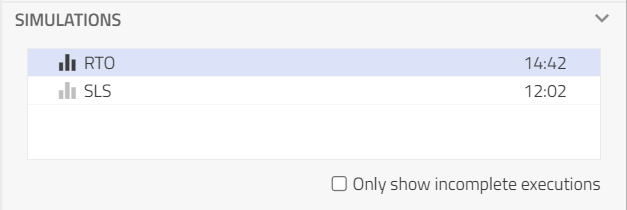
You will be automatically redirected to the Results tab and the latest results will be selected.
Displaying results🔗
Use the component views built into the library such as on design and off design to see on-design and/or off-design results.
We will additionally plot several important variables in this step.
Tip
Click here to learn how to create plots.
-
Enter pr for a pressure ratio into the search field and create a sticky for cmp and trb results.
-
Enter eff for efficiency into the search field and add compressor and turbine polytropic efficiency effPoly sticky.
-
Save the view and call it Cycle.
-
Create a sticky for one more variable nozzle gross thrust noz.Fg by searching for fg. Search for FRam in inlet and add sticky.
-
Update the Cycle view.
Tip
Click here to learn, how to create/update a view.
- The model canvas should look like below picture.
- Rename Result 1 to SLS (sea-level static).
Congratulations, you have constructed a simple turbojet model!
We see that the net thrust is still a little high in relation to our reference but we have not added bleed flows yet. Continue in the following sections to simulate any condition on the flight envelope and add bleed flows!
References🔗
Data on the J85-GE-17 from the following references are used
- Wikipedia J85 page
- Jack D. Mattingly, William H. Heiser, David T. Pratt: Aircraft Engine Design, Second edition, American Institute of Aeronautics and Astronautics, 2002.
- Edward J. Milner, Leon M. Wenzel: Performance of a J85-13 Compressor With Clean and Distorted Inlet Flow, NASA TM X-3304, 1975.
- Smithsonian Institution J85-GE-17 page
- Jeffryes W. Chapman, Thomas M. Lavelle, Jonathan S. Litt: Practical Techniques for Modeling Gas Turbine Engine Performance, NASA GRC-E-DAA-TN33214, 2017.
Different conditions🔗
This chapter will show how to set up and run off-design models at different operating conditions.
Off-Design model🔗
Firstly, we will conveniently switch the model to the off-design "mode".
- Uncheck the check box settings_JPL.onDesign via the sticky (in case you cannot see the sticky anymore, switch on the case setup stickies as described here).

Note
The equation count changes at the bottom of the canvas.

- Add compressor and turbine corrected shaft speeds and their fractions (Nc, NcqNcDes, Np, NpqNpDes) to the compressor and turbine stickies.
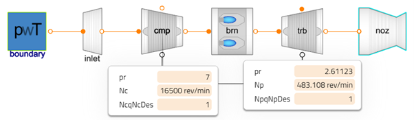
Tip
Use the off-design stickies or result mode and type "nc", "np", ... in the filter. It is also possible to use the wild card "*" to match any additional characters, so type "nc*" or "np*" for the speed fractions!
Now, we prepared the turbojet model for off-design simulation. However, the ambient conditions are still identical to the design point. So we will change them to get additional results.
Rolling takeoff🔗
We want to run the turbojet at rolling takeoff conditions. These are also called end-of-runway conditions and are typically abbreviated as RTO (or EOR).
-
Create a new experiment named RTO.
-
Change the Mach number to Mn_Par to 0.25.
-
Go to the Experimentation mode and double-check that the custom function parameter design_name is called sls (sea-level static). With this parameter, we define what sizing information to use in the off-design simulation, and we want to create off-design results for the sea-level static sizing.
-
Expand Advanced menu and select Initialize from SLS results. This means, each time we run the model, previous results will be used as guesses for the unknowns of the simulation model. This is not strictly required for this simple model but it is good practice to reuse previously converged solutions as guesses to accelerate convergence and make it more robust!
- Run the simulation and, once done, rename Result 2 to RTO.
- Check the compressor and turbine stickies and notice a slightly decreased shaft speed vs. SLS, which is expected.
Note
Rolling take-off conditions are usually simulated for hot atmospheric conditions as these are the most challenging with respect to the required thrust. In this tutorial we simplify this aspect. Look at atmosphere model parameters temperature and temperatureOffset if you are interested in the corresponding parameters.
Climb to 5000 feet🔗
-
Now, increase the altitude to 5000 ft (with same Mach Number of 0.25) and name the results Climb 5k.
-
Observe how the shaft speeds increase vs. the design value.
At 5,000 ft, the corrected shaft speed is already slightly higher than the design value. If we increase shaft speed and/or Mach Number further, the shaft speed continues to grow beyond the design value (102% at 10,000 ft, 106% at 20,000 ft with same Mach Number or 110% with Mach Number 0.5). This is usually not acceptable, and may lead to convergence issues in case the performance maps do not contain excessive shaft speeds.
Adding controls🔗
To avoid excessive shaft speeds, we will now introduce a suitable control block.
Note
If you only want to implement this basic turbojet tutorial, then you can proceed by making the suggested changes directly as described below. If you also want to implement the more advanced multi-point tutorial, then it is strongly recommended to create a new model by extending from your current experiment. Do this by right-clicking the current experiment in the left pane, and select Extend. Call the new model Controlled, and proceed as described below.
Most of the control blocks are in the package JetPropulsion.CyclePerformance.Control.
-
From the given package
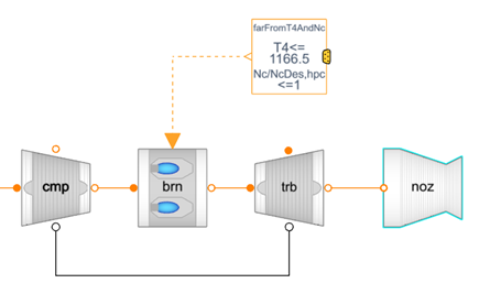
JetPropulsion.CyclePerformance.Control, drag and dropBurner.FarFromOutletTempAndSpeedto the model canvas. From the name in the package hierarchy, we can tell that this is a control block for the burner. It allows us to establish fuel flow in terms of the fuel-to-air ratio (FAR) based on thresholds on the burner outlet temperature and the shaft speed of a compressor or fan. -
Change the burner mode to fuel-to-air ratio by changing the value of switchBurn to FAR. Enable the useInput checkbox. We can now impose FAR from the control block.
-
Connect the output connector of the control block far to the input connector u of the burner. Your diagram should now look as follows.
-
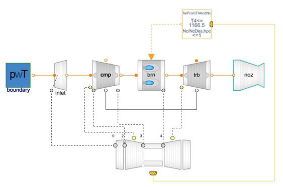
The yellow bus connector on the left of the control block still has to be connected. It represents a bus with thermodynamic station data and gas turbine metrics. In this case, we intend to read the burner outlet temperature and shaft speed from this bus. Therefore, drag
JetPropulsion.CyclePerformance.Aggregates.Turbojetinto the model. This is an aggregation component that automatically adds up gross thrust and ram drag, burner fuel flows etc. -
The station data has to be provided to the aggregation component to draw boundaries between components. Open the parameterization of the inlet, and look for the flag useSensor_a in the tab Advanced. This enables a sensor port next to inlet (port a). Enable the checkbox. Connect the sensor output sensor_a to station0 on the aggregation component with name cycleProperties.
-
Connect the remaining stations in a meaningful way. Also enable and connect the yellow compressor summary port cmpSummary and turbine summary port trbSummary. For the station definition, several alternative are possible as the compressor outlet is identical to the burner inlet. The following table lists one possibility.
| Station number | Component built-in sensor |
|---|---|
| 0 | Inlet, sensor a |
| 2 | Compressor, sensor a |
| 3 | Compressor, sensor b |
| 4 | Burner, sensor b |
-
You can now connect the yellow summary bus connectors of the aggregration component and the control block.
-
Finally, enter the nominal burner outlet temperature of 1640 °F into the parameter TtCombOutPrscrPar of the control block. Your model should now look like this.
Simulating Top Of Climb🔗
We can now simulate any reasonable Mach Number and altitude combination, as the fuel flow is throttled to avoid excessive shaft speed. To test this, and simulate top of climb (TOC) conditions, do the following.
-
In the case setup sticky, change the altitude alt_par to 35,000 ft and the Mach Number Mn_par to 0.78.
-
Go to the Experimentation mode and double check that the custom function parameter design_name is still sls (sea-level static). We will again use the sizing derived from these conditions for our simulation (in case you renamed, duplicated or extended your model since the on-design simulation, rerun this as sizing data is stored for each model separately).
-
Expand Advanced menu and select Initialize from SLS results. As before, this is not strictly required for a model as simple as this but good practice to accelerate convergence and make it more robust!
-
Run the simulation and rename Result 3 to TOC.
As expected, we see that the shaft speed limiting logic is active at TOC. The corrected shaft speed is 100% of the design value (as evident from NcqNcDes in the compressor), and the burner outlet temperature is down to approximately 1320 °F (from the nominal value of 1640 °F when the shaft speed limit is not active).
Congratulations, you have successfully used off-design steady-state solution and you have run the model at different operating conditions!
We are now able to to simulate all conditions but we have not added bleed flows yet. Continue in the following sections to improve this!
Bleed flows🔗
We will now add bleed flows to the J85 model. These bleed flow are streams of compressed air extracted from a compressor. There are many reasons for extracting bleed flows. The most important ones include the need for cooling flows for the hottest sections of the turbine, the improvement of compressor surge margin, and the provision of compressed air for other purposes onboard the aircraft such as air conditioning or anti-icing. Here, we will consider turbine cooling flows and customer bleed flows.
There is one turbine to be cooled in this turbojet. Often, we distinguish several cooling flows for each turbine. Based on how and where the cooling flow is injected, cooling pressure losses and work extraction from the flow may differ. In this simple example, we will use a typical approach and distinguish a pair of cooling flows for the turbine. Additionally, there will be one flow for customer purposes. In total, we therefore model three bleed flows from the compressor. The order shall be such that both cooling flows are covered first, and then the customer bleed flow.
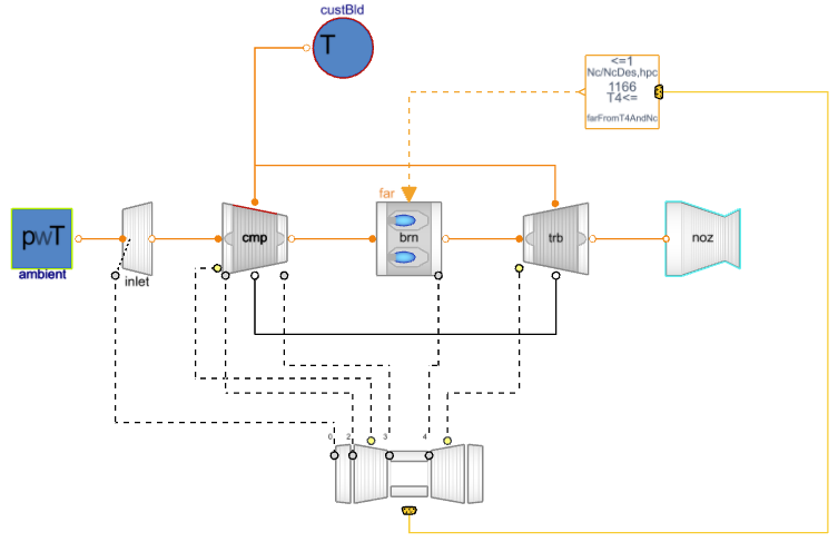
The figure is of the bleed flow model
Compressor bleed🔗
-
In the Bleed tab of the compressor parameterization, set the number of bleed ports nBld to 3.
-
For each of the three bleed ports, we must specify the position along the compressor flow path. This is done with two parameters, the relative pressure between inlet and outlet conditions fracpBld and the relative enthalpy increase between inlet and outlet fracWorkBld. Both are vectors of length nBld (i.e., three for this compressor). By default, both parameters have a vector value. We want to position all bleed ports near the outlet of the compressor. Therefore, enter {1,1,1} for both fracpBld and fracWorkBld as vector value. Next time you open the component parameterization, you can edit individual vector components as described here. You can also use the button described there to switch right away between vector and component dialog.
-
Enable wBldPrscr.
-
Finally, we can specify how much flow shall be extracted for each bleed port. This is done via variable fracwBld in relation to the total mass flow rate entering the compressor. We want to extract 5% of the total flow entering the compressor for the first cooling flow, and 2.5% for the second flow. As we do not have detailed data on the customer bleed flow requirements we set this to zero. Therefore, set fracwBld to {0.05, 0.025, 0.0}.
Tip
If you want to compute bleed flow rates physically from pressure levels and wall friction correlations, then switch off the prescription of bleed flows in the compressor. This can be done with variables wBldPrscr (all bleed ports at once) and w1BldPrscr (individually).
Turbine cooling bleed🔗
-
In the Bleed tab of the turbine parameterization, set the number of bleed ports nBld to 2.
-
For the two bleed flows, set turbineCoolingFlow to
JetPropulsion.Utilities.Types.TurbineCoolingFlow.FullandJetPropulsion.Utilities.Types.TurbineCoolingFlow.Nonerespectively, i.e., {JetPropulsion.Utilities.Types.TurbineCoolingFlow.Full, JetPropulsion.Utilities.Types.TurbineCoolingFlow.None}. -
For the cooling correlation Cooling, select Convection and film, Haselbacher.
-
For the pressure loss model PressureLossBld1 for the cooling flows contributing to the turbine work select the Nozzle Guide Vane correlation. For the pressure loss model PressureLossBld3 for the cooling flows not contributing to the turbine work select the Rotor cooling correlation.
-
You can now create connections between the compressor bleeds 1 and 2, and the turbine bleeds 1 and 2.
Customer bleed🔗
We now parameterized and connected the turbine cooling bleed. Only the customer bleed still has to be set up.
-
Drag an instance of
JetPropulsion.Boundaries.PressureBoundaryto the canvas and name it custBld. -
As we define the mass flow rate of customer bleed in the compressor (and not the sink), this is not a simple boundary condition (read the documentation embedded in the pressure boundary model to learn more). We therefore not only set isSource to false on the General tab but also switch to the Advanced tab, and set isSimple to false. This allows us to configure the boundary condition in detail. The setup is straight-forward. As we always define customer bleed pressure and mass flow rate in the compressor, set all six specify flags to false (specifypDes, specifywDes for on-design mode, specifypStdy, specifywStdy for steady-state off-design mode, specifypDyn, specifywDyn for steady-state dynamic mode). If one of the flags contains an expression by default, then simply write out false instead of disabling the checkbox.
-
You can now connect the remaining compressor bleed 3 and the customer bleed sink custBld.
Simulate design point🔗
You can now simulate again the design point, and check the results.
-
As we introduced bleed flows, the component sizing has to change. Set onDesign to true again in the settings_JPL model (use the case setup sticky to bring up this parameter quickly in case you removed it in the meantime).
-
Go to the Experimentation mode and double check that the custom function parameter design_name is still sls (sea-level static). We will use the same name for the sizing derived from the inclusion of bleed flows.
-
Run the simulation and rename Result 4 to SLS with bleed.
-
In the aggregation component cycleProperties, search for the net thrust Fn. Compare the value to the original target as sizing data is stored for each model separately).
Now the net thrust in SLS conditions is approximately 2853 lbf, and sufficiently close to the target from the reference.
Congratulations, you have successfully created a single-point turbojet design with bleed matching the J85 and simulated it in various on- and off-design operating conditions!
Continue with the bonus section or the next application tutorial to build a multi-point setup from this model.
Electrification🔗
In this section, we will install an electric motor on the turbojet shaft, to provide an extra boost of power to the engine. We will do this with components from the Electrification Library. The motivation of this section is to showcase the cross library connectivity and the application of adding an electrical system to enhance the thrust output of the engine.
Electric motor🔗
-
Add an electric motor, by dragging in an instance of
Electrification.Machines.Examples.Designonto the canvas, and name the machine em. -
Add a DC voltage supply for the motor, by dragging in an instance of
Electrification.Electrical.DCVoltageonto the canvas, and set the voltage parameter (V) to 1000 V. -
Connect the machine to the turbine, and the voltage supply to the machine.
-
(Optional) Disable the thermal connector and add a name tag on the motor, via enable_thermal_port and display_name in the Conditional tab. This makes the diagram a bit clearer, but does not affect the results.
We will now configure the controller for the machine, and add a request signal for the motor to provide 1 megawatt of mechanical power to the turbojet shaft. We will also disable the default torque and power limits, to allow us to freely design the motor output.
-
Select the machine, open the controller sub-component. Change the mode to Mechanical power control and check external_power (=true).
-
Add an instance of
Electrification.Machines.Control.Signals.pwr_refto the canvas and connect it to the machine control bus. -
Configure the pwr_ref signal component, by changing causality to parameter and specifying the value k to 1e6.
-
Select the machine, and open up the core sub-component, and the limits section. Uncheck enable_P_max and enable_tau_max. This disables the default limits that we do not care about when sizing.
Note
By default, this motor model is configured for a dynamic simulation. To allow using it for a steady state simulation, we need to disable the electrical and mechanical dynamics in the model. We will do this in the following step, by removing the supply capacitor and the rotor inertia.
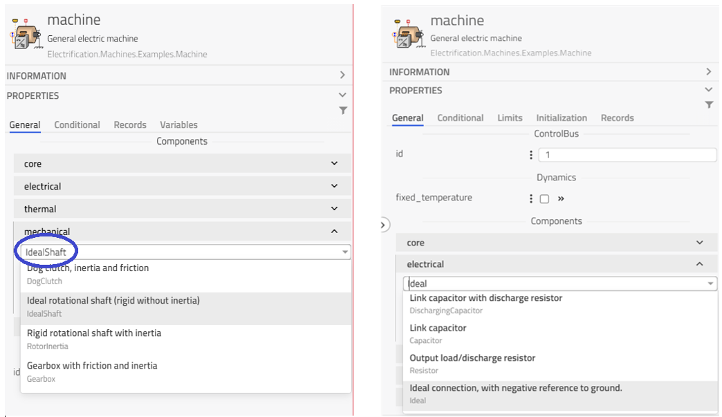
- Select the electric motor, and replace the mechanical sub-component with
Electrification.Machines.Mechanical.IdealShaft, and replace the electrical sub-component withEletrification.Machines.Electrical.Ideal.
Design🔗
This specific motor model includes sizing functionality via the design sub-component. By default, the model is configured to load an existing design from a separate design file. We will disable this to instead generate a new design, according to our specifications.
-
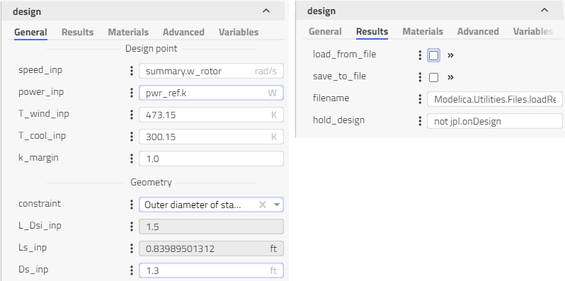
In the parameter dialog of the motor, open the design sub-component and the Results tab, and uncheck load_from_file.
-
Go back to the General tab of the design sub-component, and specify the design point power power_inp to be pwr_ref.k. This means that the motor will be designed for the maximum power corresponding to the power request signal in this experiment.
-
Also in the design sub-component, change the constraint (under Geometry) to be Outer geometry of stator, and specify the stator diameter Ds_inp to be 1.3 ft (0.4 m).
Simulate design point🔗
We will now simulate a new design point for the engine with electric motor.
-
Ensure you have configured onDesign to true in settings_JPL.
-
Go to the Experimentation mode and change the custom function parameter design_name to sls_em (to store this design with a different name than the one without electric motor).
-
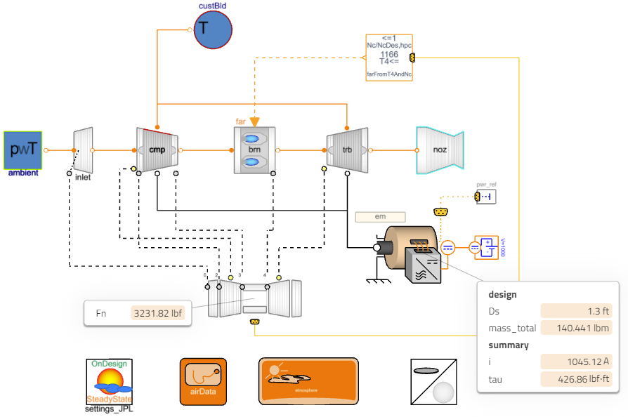
Run the simulation and rename the result to SLS electrified, and compare the change in net thrust (the variable Fn in the aggregation component cycleProperties).
You should find that the engine thrust (in SLS conditions) has increased by roughly 13 % (approximately 3232 lbf) with the addition of the electric motor. Note that the electrical setup used here is parameterized arbitrarily and hence we witness quite a small increase in thrust.
- You can look at the torque output from the motor and the electric current consumption via the variables em.summary.tau and em.summary.i. And you can look at the mass of the electric motor that we have designed, via the variable em.design.mass_total.
Congratulations, you have successfully electrified the turbojet!