OPTIMICA Compiler Toolkit🔗
The OPTIMICA Compiler Toolkit (OCT) is the calculation engine (both compiler and solver) used by Modelon Impact. It comes with a Modelica compiler with capabilities beyond dynamic simulation by offering unique features for optimization and steady-state computations.
Main features🔗
- A Modelica compiler compliant with the Modelica language specification (MLS) 3.4 supporting both Modelica Standard Library (MSL) 3.2.3-build3 as well as the Modelica Standard Library version 4.0.0 with the following exception: The language elements described in the MLS, chapter 16- Synchronous Language Elements and chapter 17 - State Machines, are not supported.
- The compiler generates Functional Mock-up Units (FMUs), including Model Exchange and Co-simulation as well as version 1.0 and 2.0 of the FMI standard.
- Dynamic simulation algorithms for integration of large-scale and stiff systems. Algorithms include CVode and Radau.
- Dynamic optimization algorithms based on collocation for solving optimal control and estimation problems. Dynamic optimization problems are encoded in Optimica, an extension to Modelica.
- A derivative-free model calibration algorithm to estimate model parameters based on measurement data.
- A non-linear solver for solving large-scale systems of equations arising, e.g., in steady-state applications. Efficient and robust steady-state problem formulation is enable by Physics Based Solving, which enables user specified selection of residuals and iteration variables.
- Support for encrypted and licensed Modelica libraries.
- Support for state-of-the-art numerical algorithms for dynamic optimization, notably the HSL solver MA57 which provides improved robustness and performance.
- A compiler API is available to extract information and manipulate, e.g., packages, models, parameters and annotations, from Modelica libraries.
- Scripting APIs in Python is available to script automation of compilation, simulation and optimization of Modelica and FMI models.
- Support for Python 3.9 on Linux and Python 3.7 on Windows.
Working with Models in Python🔗
Introduction to models🔗
Modelica and Optimica models can be compiled and loaded as model objects using the OCT Python interface. These model objects can be used for both simulation and optimization purposes. This chapter will cover how to compile Modelica and Optimica models, set compiler options, load the compiled model in a Python model object and use the model object to perform model manipulations such as setting and getting parameters.
The different model objects in OCT🔗
There are several different kinds of model objects that can be created with OCT: FMUModel(ME/CS)(1/2) (i.e. FMUModelME1, FMUModelCS1, FMUModelME2, and FMUModelCS2) and OptimizationProblem. The FMUModel(ME/CS)(1/2) is created by loading an FMU (Functional Mock-up Unit), which is a compressed file compliant with the FMI (Functional Mock-up Interface) standard. The OptimizationProblem is created by transferring an optimization problem into the CasADi-based optimization tool chain.
FMUs are created by compiling Modelica models with OCT, or any other tool supporting FMU export. OCT supports export of FMUs for Model Exchange (FMU-ME) and FMUs for Co-Simulation (FMU-CS), version 1.0 and 2.0. Import of FMU-CS version 2.0 is also supported. Generated FMUs can be loaded in an FMUModel(ME/CS) (1/2) object in Python and then be used for simulation purposes. Optimica models can not be compiled into FMUs.
OptimizationProblem objects for CasADi optimization do not currently have a corresponding file format, but are transferred directly from the OCT compiler, based on Modelica and Optimica models. They contain a symbolic representation of the optimization problem, which is used with the automatic differentiation tool CasADi for optimization purposes. Read more about CasADi and how an OptimizationProblem object can be used for optimization in Simulations of FMUs in Python.
Compilation🔗
This section brings up how to compile a model for an FMU-ME / FMU-CS. Compiling a model to an FMU-ME / FMU-CS will be demonstrated in Simple FMU-ME compilation example and Simple FMU-CS compilation example respectively.
For more advanced usage of the compiler functions, there are compiler options and arguments which can be modified. These will be explained in Compiler settings.
Simple FMU-ME compilation example🔗
The following steps compile a model to an FMU-ME version 2.0:
- Import the OCT compiler function compile_fmu from the package pymodelica.
- Specify the model and model file.
- Perform the compilation.
This is demonstrated in the following code example:
#Import the compiler function
from pymodelica import compile_fmu

# Specify Modelica model and model file (.mo or .mop)
model_name = 'myPackage.myModel'
mo_file = 'myModelFile.mo'

# Compile the model and save the return argument, which is the file name of the FMU
my_fmu = compile_fmu(model_name, mo_file)
There is a compiler argument target that controls whether the model will be exported as an FMU-ME or FMU-CS. The default is to compile an FMU-ME, so target does not need to be set in this example. The compiler argument version specifies if the model should be exported as an FMU 1.0 or 2.0. As the default is to compile an FMU 2.0, version does not need to be set either in this example. To compile an FMU 1.0, version should be set to '1.0'.
Once compilation has completed successfully, an FMU-ME 2.0 will have been created on the file system. The FMU is essentially a compressed file archive containing the files created during compilation that are needed when instantiating a model object. Return argument for compile_fmu is the file path of the FMU that has just been created, this will be useful later when we want to create model objects. More about the FMU and loading models can be found in Loading models.
In the above example, the model is compiled using default arguments and compiler options - the only arguments set are the model class and file name. However, compile_fmu has several other named arguments which can be modified. The different arguments, their default values and interpretation will be explained in Compiler settings.
Simple FMU-CS compilation example🔗
The following steps compiles a model to an FMU-CS version 2.0:
-
Import the OCT compiler function compile_fmu from the package pymodelica.
-
Specify the model and model file.
-
Set the argument target = 'cs'
-
Perform the compilation.
This is demonstrated in the following code example:
# Import the compiler function
from pymodelica import compile_fmu

# Specify Modelica model and model file (.mo or .mop)
model_name = 'myPackage.myModel'
mo_file = 'myModelFile.mo'

# Compile the model and save the return argument, which is the file name of the FMU
my_fmu = compile_fmu(model_name, mo_file, target='cs')
In a Co-Simulation FMU, the integrator for solving the system is contained within the FMU. With an FMU-CS exported with OCT, three different solvers are supported: CVode, Explicit Euler, Radau5 and Runge-Kutta (2nd order).
Compiling from libraries🔗
The model to be compiled might not be in a standalone .mo file, but rather part of a library consisting of a directory structure containing several Modelica files. In this case, the file within the library that contains the model should not be given on the command line. Instead, the entire library should to added to the list of libraries that the compiler searches for classes in. This can be done in several ways (here library directory refers to the top directory of the library, which should have the same name as the top package in the library):
• Giving the path to the library directory in the file_name argument of the compilation function. This allows adding a specific library to the search list (as opposed to adding all libraries in a specific directory).
• Set the directory containing a library directory via the keyword argument named modelicapath of the compilation function. This allows for adding several libraries to the search list. For example if modelicapath=C : \MyLibs, then the compiler sets MODELICAPATH to C : \MyLibs and all libraries within are added to the search list during compilation.
The Modelica Standard Library (MSL) that is included in the installation is loaded by default, when starting the OCT Python shell . The version of MSL that is loaded is added on the compiler option named msl_version or any existing uses annotations within the model being compiled.
The Python code example below demonstrates these methods:
# Import the compiler function
from pymodelica import compile_fmu

# Compile an example model from the MSL
fmu1 = compile_fmu('Modelica.Mechanics.Rotational.Examples.First')

# Compile an example model utilizing the modelica path keyword argument assuming
# the library MyLibrary is located in C:/MyLibs, i.e. C:/MyLibs/MyLibrary exists
fmu2 = compile_fmu('MyLibrary.MyModel', 'C:/MyLibs/MyLibrary')
Compiler settings🔗
The compiler function arguments can be listed with the interactive help in Python. The arguments are explained in the corresponding Python docstring which is visualized with the interactive help. This is demonstrated for compile_fmu below. The docstring for any other Python function for can be displayed in the same way.
compile_fmu arguments🔗
The compile_fmu arguments can be listed with the interactive help.
# Display the docstring for compile_fmu with the Python command 'help'
from pymodelica import compile_fmu
help(compile_fmu)
Help on function compile_fmu in module pymodelica.compiler:

compile_fmu(class_name, file_name = [], compiler = 'auto',
        target = 'me', version = '2.0', platform =  'auto',
        compiler_options = {}, compile_to = '.',
        compiler_log_level = 'warning',
        modelicapath = ' ',  separate_process = True, jvm_args = '') :
Compile a Modelica model to an FMU.

A model class name must be passed, all other arguments have default values.
The different scenarios are:

* Only class_name is passed:
    - Class is assumed to be in MODELICAPATH.

* class_name and file_name is passed:
    - file_name can be a single path as a string or a list of paths
 (strings). The paths can be file or library paths.
    - Default compiler setting is 'auto' which means that the appropriate
    compiler will be selected based on model file ending, i.e.
    ModelicaCompiler if a .mo file and OptimicaCompiler if a .mop file is
    found in file_name list.

The compiler target is 'me' by default which means that the shared
file contains the FMI for Model Exchange API. Setting this parameter to
'cs' will generate an FMU containing the FMI for Co-Simulation API.

Parameters::

    class_name --
        The name of the model class.

    file_name --
        A path (string) or paths (list of strings) to
        model files and/or libraries. If file does not exist,an exception of
        type pymodelica.compiler_exceptions.PyModelicaFileError is raised.
        Default: Empty list.

    compiler --
        The compiler used to compile the model. The different options are:
        - 'auto': the compiler is selected automatically depending on file ending
        - 'modelica': the ModelicaCompiler is used
        - 'optimica': the OptimicaCompiler is used
        Default: 'auto'

    target --
        Compiler target. Possible values are 'me', 'cs' or 'me+cs'.
        Default: 'me'

    version --
        The FMI version. Valid options are '1.0' and '2.0'.
        Default: '2.0'

    platform --
        Set platform, controls whether a 32 or 64 bit FMU is generated.
        This option is only available for Windows.
        Valid options are :
        - 'auto': platform is selected automatically.
        This is the only valid option for linux & darwin.
        - 'win32': generate a 32 bit FMU
        - 'win64': generate a 64 bit FMU
        Default: 'auto'


    compiler_options --
        Options for the compiler.
        Default: Empty dict.

    compile_to --
        Specify target file or directory. If file, any intermediate directories
        will be created if they don't exist. Furthermore, the modelica model
        will be renamed to this name. If directory, the path given
        must exist and the model will keep its original name.
        Default: Current directory.

    compiler_log_level --
        Set the logging for the compiler. Takes a comma separated list with
        log outputs. Log outputs start with a flag :'warning'/'w',
        'error'/'e', 'verbose'/'v', 'info'/'i' or 'debug'/'d'.
        The log can be written to file
        by appended flag with a colon and file name.
        Example: compiler_log_level='d:debug.txt', sets the log level to debug
        and writes the log to a file named  'debug.txt'
        Default: 'warning'

    separate_process --
        Run the compilation of the model in a separate process.
        Checks the environment variables (in this order):
            1. SEPARATE_PROCESS_JVM
            2. JAVA_HOME
        to locate the Java installation to use.
        For example (on Windows) this could be:
            SEPARATE_PROCESS_JVM = C:\Program Files\Java\jdk1.6.0_37
        Default: True

    jvm_args --
        String of arguments to be passed to the JVM when compiling in a
        separate process.
        Default: Empty string

Returns::
    A compilation result, represents the name of the FMU which has been
    created and a list of warnings that was raised.
Compiler options🔗
Compiler options can be modified using the compile_fmu argument compiler_options. This is shown in the example below.
# Compile with the compiler option 'enable_variable_scaling' set to True
# Import the compiler function
from pymodelica import compile_fmu

# Specify model and model file
model_name = 'myPackage.myModel'
mo_file = 'myModelFile.mo'

# Compile
my_fmu = compile_fmu(model_name, mo_file,
 compiler_options={"enable_variable_scaling":True})
There are four types of options: string, real, integer and boolean. The complete list of options can be found in Appendix B in the OPTIMICA Compiler Toolkit User's guide
Loading models🔗
Compiled models, FMUs, are loaded in the OCT Python interface with the FMUModel(ME/CS) (1/2) class from the pyfmi module, while optimization problems for the CasADi-based optimization are transferred directly into the OptimizationProblem class from the pyjmi module. This will be demonstrated in Loading an FMU and Transferring an Optimization Problem. The model classes contain many methods with which models can be manipulated after instantiation. Among the most important methods are initialize and simulate, which are used when simulating. These are explained in Simulations of FMUs in Python and Dynamic Optimization in Python. For more information on how to use the OptimizationProblem for optimization purposes, see Dynamic Optimization in Python. The more basic methods for variable and parameter manipulation are explained in Changing model parameters.
Loading an FMU🔗
An FMU file can be loaded in OCT with the method load_fmu in the pyfmi module. The following short example demonstrates how to do this in a Python shell or script.
# Import load_fmu from pyfmi
from pyfmi import load_fmu
myModel = load_fmu('myFMU.fmu')
load_fmu returns a class instance of the appropriate FMU type which then can be used to set parameters and used for simulations.
Transferring an Optimization Problem🔗
An optimization problem can be transferred directly from the compiler in OCT into the class OptimizationProblem in the pyjmi module. The transfer is similar to the combined steps of compiling and then loading an FMU. The following short example demonstrates how to do this in a Python shell or script.
# Import transfer_optimization_problem
from pyjmi import transfer_optimization_problem

# Specify Modelica model and model file
model_name = 'myPackage.myModel'
mo_file = 'myModelFile.mo'

# Compile the model, return argument is an OptimizationProblem
myModel = transfer_optimization_problem(model_name, mo_file)
Changing model parameters🔗
Model parameters can be altered with methods in the model classes once the model has been loaded. Some short examples in Setting and getting parameters will demonstrate this.
Setting and getting parameters🔗
The model parameters can be accessed via the model class interfaces. It is possible to set and get one specific parameter at a time or a whole list of parameters.
The following code example demonstrates how to get and set a specific parameter using an example FMU model from the pyjmi.examples package.
# Compile and load the model
from pymodelica import compile_fmu
from pyfmi import load_fmu
my_fmu = compile_fmu('RLC_Circuit','RLC_Circuit.mo')
rlc_circuit = load_fmu(my_fmu)

# Get the value of the parameter 'resistor.R' and save the result in a variable
 'resistor_r'
resistor_r = rlc_circuit.get('resistor.R')

# Give 'resistor.R' a new value
resistor_r = 2.0
rlc_circuit.set('resistor.R', resistor_r)
The following example demonstrates how to get and set a list of parameters using the same example model as above. The model is assumed to already be compiled and loaded.
# Create a list of parameters, get and save the corresponding values in a variable 'values'
vars = ['resistor.R', 'resistor.v', 'capacitor.C', 'capacitor.v']
values = rlc_circuit.get(vars)
# Change some of the values
values[0] = 3.0
values[3] = 1.0
rlc_circuit.set(vars, values)
Debugging models🔗
The OCT compilers can generate debugging information in order to facilitate localization of errors. There are three mechanisms for generating such diagnostics: dumping of debug information to the system output, generation of HTML code that can be viewed with a standard web browser or logs in XML format from the non-linear solver.
Compiler logging🔗
The amount of logging that should be output by the compiler can be set with the argument compiler_log_level to the compile-functions (compile_fmu and also transfer_optimization_problem). The available log levels are 'warning' (default), 'error', 'info', 'verbose' and 'debug' which can also be written as 'w', 'e', 'i', 'v' and 'd' respectively. The following example demonstrates setting the log level to 'info':
# Set compiler log level to 'info'
compile_fmu('myModel', 'myModels.mo', compiler_log_level='info')
The log is printed to the standard output, normally the terminal window from which the compiler is invoked.
The log can also be written to file by appending the log level flag with a colon and file name. This is shown in the following example:
# Set compiler log level to info and write the log to a file log.txt
compile_fmu('myModel', 'myModels.mo', compiler_log_level='i:log.txt')
It is possible to specify several log outputs by specifying a comma separated list. The following example writes log warnings and errors (log level 'warning' or 'w') to the standard output and a more verbose logging to file (log level 'info' or 'i'):
# Write warnings and errors to standard output and the log with log level info to log.txt
compile_fmu('myModel', 'myModels.mo', compiler_log_level= 'w,i:log.txt')
Runtime logging🔗
Runtime logging refers to logging of data during simulation, this section outlines some methods to retrieve simulation data from an FMU.
Setting log level🔗
Many events that occur inside of an FMU can generate log messages. The log messages from the runtime are saved
in a file with the default name
# Load model
model = load_fmu(fmu_name, log_file_name='MyLog.txt')
How much information that is output to the log file can be controlled by setting the log_level argument to load_fmu. log_level can be any number between 0 and 7, where 0 means no logging and 7 means the most verbose logging. The log level can also be changed after the FMU has been loaded with the function set_log_level(level). Setting the log_level is demonstrated in the following example:
# Load model and set log level to 5
model = load_fmu(fmu_name, log_level=5)
# Change log level to 7
model.set_log_level(7)
If the loaded FMU is an FMU exported by OCT, the amount of logging produced by the FMU can also be altered. This is done by setting the parameter _log_level in the FMU. This log level ranges from 0 to 7 where 0 represents the least verbose logging and 7 the most verbose. The following example demonstrates this:
# Load model (with default log level)
model = load_fmu(fmu_name)
# Set amount of logging produced to the most verbose
model.set('_log_level', 6)
# Change log level to 7 to be able to see everything that is being produced
model.set_log_level(7)
Interpreting logs from FMUs produced by OCT🔗
In OCT, information is logged in XML format, which ends up mixed with FMI Library output in the resulting log file. Example: (the following examples are based on the example pyjmi.examples.logger_example.)
 1 ...
 2 FMIL: module = FMICAPI, log level = 5: Calling fmiInitialize
 3 FMIL: module = Model, log level = 4: [INFO][FMU status:OK] <EquationSolve>Model equations evaluation invoked at<value name="t"> 0.0000000000000000E+00</value>
 4 FMIL: module = Model, log level = 4: [INFO][FMU status:OK] <BlockEventIterations>Starting block (local) event iteration at<value name="t"> 0.0000000000000000E+00</value>in<value name="block">0</value>
 5 FMIL: module = Model, log level = 4: [INFO][FMU status:OK] <vector name="ivs"> 0.0000000000000000E+00, 0.0000000000000000E+00, 0.0000000000000000E+00<vector>
 6 FMIL: module = Model, log level = 4: [INFO][FMU status:OK] <vector name="switches">0.0000000000000000E+00, 0.0000000000000000E+00, 0.0000000000000000E+00, 0.0000000000000000E+00</vector>
 7 FMIL: module = Model, log level = 4: [INFO][FMU status:OK] <vectorname="booleans"></vector>
 8 FMIL: module = Model, log level = 4: [INFO][FMU status:OK] <BlockIteration>Localiteration<value name="iter">1</value>at<value name="t"> 00000000000000000E+00</value>
 9 FMIL: module = Model, log level = 4: [INFO][FMU status:OK] <JacobianUpdated><value name="block">0</value>
 10 FMIL: module = Model, log level = 4: [INFO][FMU status:OK] <matrixname="jacobian">
 11 FMIL: module = Model, log level = 4: [INFO][FMU status:OK] -1.0000000000000000E+00, 4.0000000000000000E+00, 0.0000000000000000E+00;
 12 FMIL: module = Model, log level = 4: [INFO][FMU status:OK] -1.0000000000000000E+00, -1.0000000000000000E+00, -1.0000000000000000E+00;
 13 FMIL: module = Model, log level = 4: [INFO][FMU status:OK] -1.0000000000000000E+00, 1.0000000000000000E+00, -1.0000000000000000E+00;
 14 FMIL: module = Model, log level = 4: [INFO][FMU status:OK] </matrix>
 15 FMIL: module = Model, log level = 4: [INFO][FMU status:OK] </JacobianUpdated>
 16 ...
The log can be inspected manually, using general purpose XML tools, or parsed using the tools in pyfmi.common.log. A pure XML file that can be read by XML tools can be extracted with
# Generate an XML file from the simulation log that
was generated by model.simulate()
model.extract_xml_log()
The XML contents can also be parsed directly:
# Parse the entire XML log
log = pyfmi.common.log.parse_fmu_xml_log(log_file_name)
log will correspond to the top level log node, containing all other nodes. Log nodes have two kinds of children: named (with a name attribute in the XML file) and unnamed (without).
• Named children are accessed by indexing with a string: node['t'], or simply dot notation: node.t.
• Unnamed children are accessed as a list node.nodes, or by iterating over the node.
There is also a convenience function gather_solves to extract common information about equation solves in the log. This function collects nodes of certain types from the log and annotates some of them with additional named children. The following example is from pyjmi.examples.logger_example:
 1 # Parse the entire XML log
 2 log = pyfmi.common.log.parse_fmu_xml_log(log_file_name)
 3 # Gather information pertaining to equation solves
 4 solves = pyjmi.log.gather_solves(log)
 5
 6 print('Number of solver invocations:', len(solves))
 7 print('Time of first solve:', solves[0].t)
 8 print('Number of block solves in first solver invocation:', len(solves[0].block_solves)
 9 print('Names of iteration variables in first block solve:',
 solves[0].block_solves[0].variables))
 10 print('Min bounds in first block solve:',
 solves[0].block_solves[0].min)
 11 print('Max bounds in first block solve:',
 solves[0].block_solves[0].max)
 12 print('Initial residual scaling in first block solve:',
 solves[0].block_solves[0].initial_residual_scaling)
 13 print('Number of iterations in first block solve:',
 len(solves[0].block_solves[0].iterations)
 14 print('\n')
 15 print('First iteration in first block solve: ')
 16 print(' Iteration variables:',
 solves[0].block_solves[0].iterations[0].ivs)
  17 print(' Scaled residuals:',
 solves[0].block_solves[0].iterations[0].residuals)
 18 print(' Jacobian:\n',
 solves[0].block_solves[0].iterations[0].jacobian)
 19 print(' Jacobian updated in iteration:',
 solves[0].block_solves[0].iterations[0].jacobian_updated)
 20 print(' Residual scaling factors:',
 solves[0].block_solves[0].iterations[0].residual_scaling)
 21 print(' Residual scaling factors_updated:',
 solves[0].block_solves[0].iterations[0].residual_scaling_updated)
 22 print(' Scaled residual norm:',
 solves[0].block_solves[0].iterations[0].scaled_residual_norm)
Compiler Diagnostic Output🔗
By setting the compiler option generate_html_diagnostics to true, a number of HTML pages containing diagnostics are generated. The HTML files are generated in the directory Model_Name_diagnostics, where Model_Name is the name of the compiled model. As compared to the diagnostics generated by the compiler_log_level argument, the HTML diagnostics contains only the most important information, but it also provides a better overview. Opening the file Model_Name_diagnostics/index.html in a web browser, results in a page with information on number of variables, parameters and equations as well as other statistics about the model.
Note that some of the entries in Model_Name_diagnostics/index.html, including Problems, Flattened model, Connection sets, Transformed model, Alias sets, BLT diagnostics table, BLT for DAE System and BLT for Initialization System are links to sub pages containing additional information. For example, the BLT for DAE System page contains information about in which order the model equations are evaluated and which blocks are present after compilation.
Additionally there is a table view of the BLT. It can be found on the BLT diagnostics table page. It provides a graphical representation of the BLT. The BLT diagnostics table is only generated when the model have fewer equations than the limit specified by the option diagnostics_limit due to the size of the graph.
In the following section a more thorough description of the HTML diagnostics will be presented.
HTML diagnostics🔗
The compiler can generate diagnostic output in HTML format which can be viewed in, e.g, a web browser. The generation is enabled through the option generate_html_diagnostics and the diagnostic consists of several pages which will be presented in the sections below.
index.html
index.html is the index page or, i.e., the start page of the HTML diagnostics. It consists of links to the other diagnostic pages as well as statistics of the compiled model. Model before transformation summarizes model statistics of the flattened model. Model after transformation gives the statistics after the compiler has done its transformations to the model like, for example, alias elimination. Finally the number of unsolved equation blocks in DAE initialization system and system before and after tearing is applied is presented. Note that nested blocks are not visible in the equation block statistics.
errors.html
The page errors.html, which can be reached from Problems in the index page, lists all compiler errors and warnings that occurred during compilation.
flattened.html
In flattened.html, the flattened model, which the numbers in Model before transformation corresponds to, is presented. That includes a listing of all constants, parameters and variables in the model with their type_prefix, type_specifier, the possible array subscripts, and the fully qualified name. If the type_specifier is not a built-in type, the defined type will be presented at the end of the page like, e.g.,
type Modelica.Units.SI.MassFraction = Real(final quantity = "MassFraction",final unit = "1",min = 0,max = 1);
After all the components, the initial equations are presented followed by the equations in the order they are read in by the compiler. Note that the components are given by their fully qualified name. When functions are used in the model, the function description with its inputs, outputs and algorithm is given in the end of the page. Definitions of records used in the model can be found there as well.
Note that uses of constants, e.g., Modelica.Constants.pi, in
parameter Real x=Modelica.Constants.pi;
will have been evaluated (to 3.141592653589793) when declared in the flattened model. This is also true for parameters and variables which are necessary to evaluate (for example parameters used as array sizes) or determined to be equivalent to constants (for example a final independent parameter).
transformed.html
he transformed model, presented in transformed.html, has the same structure as the flattened model. The numbers in Model after transformation corresponds to this stage of the compilation process. In the transformed model alias variables are removed, temporary variables are introduced and some other symbolic transformations are performed. Furthermore, extra initial equations may have been introduced based on, e.g., start attributes set on variables.
alias.html
In alias.html alias variables are listed set by set. Each set is enclosed within curly brackets and the first variable in the list is the variable name used in the transformed model.
blt.html and initBlt.html
In initBlt.html and blt.html all the equations are sorted in the order in which they are calculated, i.e., by causality. The initialization system is found in initBlt.html and the BLT for the DAE system in blt.html. In case of an interactive FMU, these two systems coincide.
The BLT consists of solved equations, meta equations and different kinds of blocks. For equations below the Solved equation label, the variable on the left hand side is calculated directly through evaluation of the right hand side. Meta equation blocks hold assert statements etc.
Blocks can be linear, non-linear as well as having discrete parts. The block type is documented in the title, for example, Torn system (Block 1) of 1 iteration variables and 3 solved variables. Included in the title is also the name of the block, which in turn is used in the runtime logging. Continuous iteration variables, torn variables and discrete variables are listed in separate columns. So are also the equations corresponding to each of the categories.
When reading the BLT from the interactive FMU perspective, res_i, with i=0,1,2..., corresponds to the residual equations. There is no easy way to detect which variables are the iteration variables of the steady state problem from this view. Nestled blocks will be presented as blocks are presented for segregated FMUs, before the residual equations, since these are to be solved before the residuals can be evaluated.
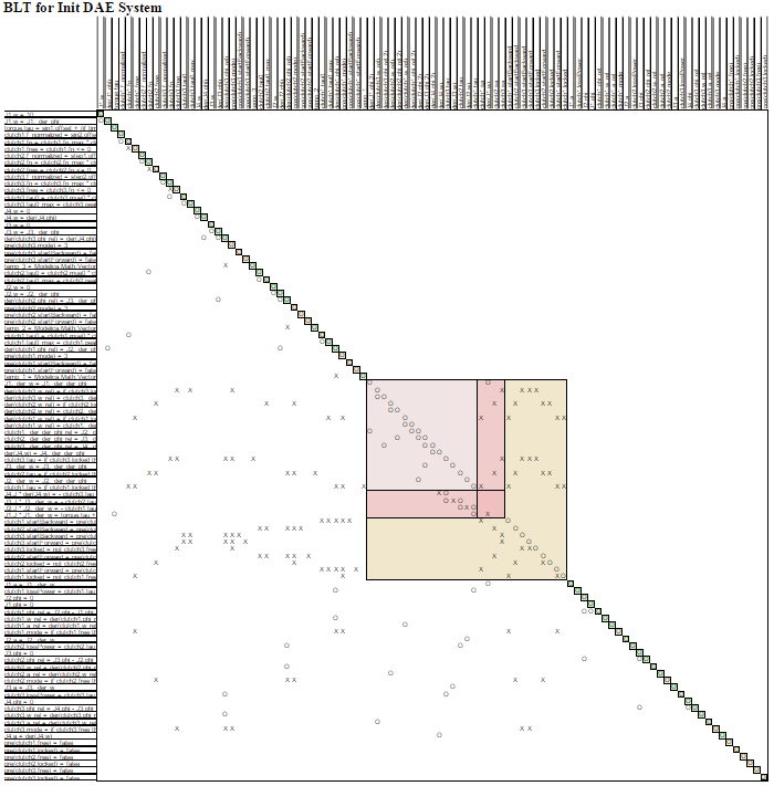
bltTable.html
The relationship between the equations and the variables is presented in bltTable.html. As for the BLT, there exist two tables: one for the initialization system and one for the DAE system. Even for this case, the tables are the same for an interactive FMU.
In the table, the equations are listed in the rows and the variables in the columns. The equation appears in the same form as in transformed.html. There are different colors and symbols in the BLT table. We have
| o | The 'o' means that the variable is analytically solvable from the equation if all the other variables are known. |
| x | The 'x' means that the variable cannot be solved for analytically even if the other variables are known. |
| green | The green color marks a solved equation. |
| pink | A pink block shows algebraic equation blocks |
| dark pink | The dark pink highlights the iteration variables and residual equations of the lighter pink block. |
| orange | The orange color marks discrete equations and variables. |
| blue | The blue color marks an equation block where all equations are unsolved. |
An example of how the BLT table may look like can be found in Figure 4.1. Note that a legned is also generated in the BLT with an explanation of the symbols.
Simulations of FMUs in Python🔗
Introduction🔗
OCT supports simulation of models described in the Modelica language and models following the FMI standard. The simulation environment uses Assimulo as standard which is a standalone Python package for solving ordinary differential and differential algebraic equations. Loading and simulation of FMUs has additionally been made available as a separate Python package, PyFMI.
This chapter describes how to load and simulate FMUs using explanatory examples.
A first example🔗
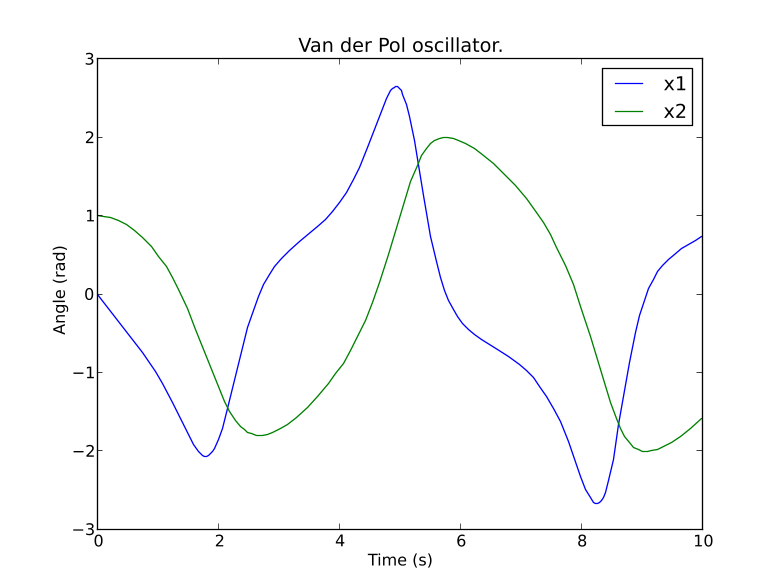
This example focuses on how to use OCT's simulation functionality in the most basic way. The model which is to be simulated is the Van der Pol problem described in the code below. The model is also available from the examples in OCT in the file VDP.mop (located in install/Python/pyjmi/examples/files).
model VDP
    // State start values
    parameter Real x1_0 = 0;
    parameter Real x2_0 = 1;

    // The states
    Real x1(start = x1_0);
    Real x2(start = x2_0);

    // The control signal
    input Real u;

 equation
    der(x1) = (1 - x2^2) * x1 - x2 + u;
    der(x2) = x1;
end VDP;
Create a new file in your working directory called VDP.mo and save the model.
Next, create a Python script file and write (or copy paste) the commands for compiling and loading a model:
# Import the function for compilation of models and the load_fmu method
from pymodelica import compile_fmu
from pyfmi import load_fmu

# Import the plotting library
import matplotlib.pyplot as plt

# Compile model
fmu_name = compile_fmu("VDP","VDP.mo")
# Load model
vdp = load_fmu(fmu_name)
The function compile_fmu compiles the model into a binary, which is then loaded when the vdp object is created. This object represents the compiled model, an FMU, and is used to invoke the simulation algorithm (for more information about model compilation and options, see Working with Models in Python:
res = vdp.simulate(final_time=10)
In this case we use the default simulation algorithm together with default options, except for the final time which we set to 10. The result object can now be used to access the simulation result in a dictionary-like way:
x1 = res['x1']
x2 = res['x2']
t = res['time']
The variable trajectories are returned as NumPy arrays and can be used for further analysis of the simulation result or for visualization:
plt.figure(1)
plt.plot(t, x1, t, x2)
plt.legend(('x1','x2'))
plt.title('Van der Pol oscillator.')
plt.ylabel('Angle (rad)')
plt.xlabel('Time (s)')
plt.show()
Simulation of Models🔗
Simulation of models in OCT is performed via the simulate method of a model object. The FMU model objects in OCT are located in PyFMI:
• FMUModelME1 / FMUModelME2
• FMUModelCS1 / FMUModelCS2
FMUModelME * / FMUModelCS * also supports compiled models from other simulation/modelling tools that follow the FMI standard (extension .fmu) (either Model exchange FMUs or Co-Simulation FMUs). Both FMI version 1.0 and FMI version 2.0 are supported. For more information about compiling a model in OCT see Working with Models in Python.
The simulation method is the preferred method for simulation of models and which by default is connected to the Assimulo simulation package but can also be connected to other simulation platforms. The simulation method for FMUModelME * / FMUModelCS * is defined as:
class FMUModel(ME/CS)(...)
    ...
    def simulate(self,
            start_time=0.0,
            final_time=1.0,
            input=(),
            algorithm='AssimuloFMIAlg',
            options={}):
And used in the following way:
res = FMUModel(ME/CS)*.simulate() # Using default values
For FMUModelCS *, the FMU contains the solver and is thus used (although using the same interface)
Convenience method, load_fmu🔗
Since there are different FMI specifications for Model exchange and Co-Simulation and also differences between versions, a convenience method, load_fmu has been created. This method is the preferred access point for loading an FMU and will return an instance of the appropriate underlying FMUModel(CS/ME) * class.
Arguments🔗
The start and final time attributes are simply the time where the solver should start the integration and stop the integration. The input however is a bit more complex and is described in more detail in the following section. The algorithm attribute is where the different simulation package can be specified, however currently only a connection to Assimulo is supported and connected through the algorithm AssimuloFMIAlg for FMUModelME *.
Inputs🔗
The input argument defines the input trajectories to the model and should be a 2-tuple consisting of the names of the input variables and their trajectories. The names can be either a list of strings, or a single string for setting only a single input trajectory. The trajectories can be given as either a data matrix or a function. If a data matrix is used, it should contain a time vector as the first column, and then one column for each input, in the order of the list of names. If instead the second argument is a function it should be defined to take the time as input and return an array with the values of the inputs, in the order of the list of names.
For example, consider that we have a model with an input variable u1 and that the model should be driven by a sine wave as input. We are interested in the interval 0 to 10. We will look at both using a data matrix and at using a function.
import numpy as N
t = N.linspace(0.,10.,100) # Create one hundred evenly spaced points
u = N.sin(t) # Create the input vector
u_traj = N.transpose(N.vstack((t,u))) # Create the data matrix and transpose
                                      # it to the correct form
The above code have created the data matrix that we are interested in giving to the model as input, we just need to connect the data to a specific input variable, u1:
input_object = ('u1', u_traj)
Now we are ready to simulate using the input and simulate 10 seconds.
res = model.simulate(final_time=10, input=input_object)
If we on the other hand would have two input variables, u1 and u2 the script would instead look like:
import numpy as N
t = N.linspace(0.,10.,100)                      # Create one hundred evenly spaced points
u1 = N.sin(t)                                   # Create the first input vector
u2 = N.cos(t)                                   # Create the second input vector
u_traj = N.transpose(N.vstack((t,u1,u2)))       # Create the data matrix and
                                                # transpose it to the correct form
input_object = (['u1','u2'], u_traj)
res = model.simulate(final_time=10, input=input_object)
Options for Model Exchange FMUs🔗
The options attribute are where options to the specified algorithm are stored and are preferably used together with:
opts = FMUModelME*.simulate_options()
which returns the default options for the default algorithm. Information about the available options can be viewed by typing help on the opts variable:
>>> help(opts)
    Options for the solving the FMU using the Assimulo simulation package.
    Currently, the only solver in the Assimulo package that fully supports
    simulation of FMUs is the solver CVode.
    ...
In Table 1 the general options for the AssimuloFMIAlg algorithm are described while in Table 2 a selection of the different solver arguments for the ODE solver CVode is shown. More information regarding the solver options can be found here, www.jmodelica.org/assimulo.
| Options | Default | Description |
|---|---|---|
| solver | "CVode" | Specifies the simulation method that is to be used. Currently supported solvers are, CVode, Radau5ODE, RungeKutta34, Dopri5, RodasODE, LSODAR, ExplicitEuler. The recommended solver is "CVode". |
| ncp | 500 | Number of communication points. If ncp is zero, the solver will return the internal steps taken. |
| initialize | True | If set to True, the initializing algorithm defined in the FMU model is invoked, otherwise it is assumed the user have manually invoked model.initialize() |
| write_scaled_result | False | When true, write the result to file without taking numerical scaling into account. |
| result_file_name | Empty string (default generated file name will be used) | Specifies the name of the file where the simulation result is written. Setting this option to an empty string results in a default file name that is based on the name of the model class. |
| filter | None | A filter for choosing which variables to actually store result for. The syntax can be found here. An example is filter = "*der" , store all variables ending with 'der' and filter = ["*der*", "summary*"], store all variables with "der" in the name and all variables starting with "summary". |
| result_handling | "file" | Specifies how the result should be handled. Either stored to file or stored in memory. One can also use a custom handler. Available options: "file", "memory", "custom" |
Lets look at an example, consider that you want to simulate an FMU model using the solver CVode together with changing the discretization method (discr) from BDF to Adams:
opts = model.simulate_options()          # Retrieve the default options
#opts['solver'] = 'CVode'                # Not necessary, default solver is CVode
opts['CVode_options']['discr'] = 'Adams' # Change from using BDF to Adams
opts['initialize'] = False               # Don't initialize the model
model.simulate(options=opts)             # Pass in the options to simulate and simulate
It should also be noted from the above example that the options regarding a specific solver, say the tolerances for CVode, should be stored in a double dictionary where the first is named after the solver concatenated with _options:
opts['CVode_options']['atol'] = 1.0e-6 # Options specific for CVode
For the general options, as changing the solver, they are accessed as a single dictionary:
opts['solver'] = 'CVode' # Changing the solver
opts['ncp'] = 1000       # Changing the number of communication points.
| Option | Default | Description |
|---|---|---|
| disc | 'BDF' | Discretization method. Can be either 'BDF' or 'Adams'. |
| iter | 'Newton' | The iteration method. Can be either 'Newton' or 'FixedPoint'. |
| maxord | 5 | The maximum order used. Maximum for 'BDF' is 5 while for the 'Adams' method the maximum is 12. |
| minh | 0.0 | Minimal step-size. |
| maxh | Inf | Maximum step-size. |
| rtol | 1e-4 | Relative tolerance. The relative tolerance is retrieved from the 'default experiment' section in the XMLfile and if not found is set to 1.0e-4. |
| atol | rtol*0.01*(nominal values of the continuous states) | Absolute Tolerance. Can be an array where each value corresponds to the absolute tolerance for the corresponding variable. Can also be a single value. |
Options for Co-Simulation FMUs🔗
The options attribute are where options to the specified algorithm are stored, and are preferably used together with:
opts = FMUModelCS*.simulate_options()
which returns the default options for the default algorithm. Information about the available options can be viewed by typing help on the opts variable:
>>> help(opts)
 Options for the solving the CS FMU.

 ...
In Table 3 the general options for the FMICSAlg algorithm are described.
| Options | Default | Description |
|---|---|---|
| ncp | 500 | Number of communication points. If ncp is zero, the solver will return the internal steps taken. |
| initialize | True | If set to True, the initializing algorithm defined in the FMU model is invoked, otherwise it is assumed the user have manually invoked model.initialize() |
| write_scaled_result | False | When true, write the result to file without taking numerical scaling into account. |
| result_file_name | Empty string (default generated file name will be used) | Specifies the name of the file where the simulation result is written. Setting this option to an empty string results in a default file name that is based on the name of the model class. |
| filter | None | A filter for choosing which variables to actually store result for. The syntax can be found here. An example is filter = "*der" , store all variables ending with 'der' and filter = ["*der*", "summary*"], store all variables with "der" in the name and all variables starting with "summary". |
| result_handling | "file" | Specifies how the result should be handled. Either stored to file or stored in memory. One can also use a custom handler. Available options: "file", "memory", "custom" |
Return argument🔗
The return argument from the simulate method is an object derived from a common result object ResultBase in algorithm_drivers.py with a few extra convenience methods for retrieving the result of a variable. The result object can be accessed in the same way as a dictionary type in Python with the name of the variable as key.
res = model.simulate()
y = res['y']           # Return the result for the variable/parameter/constant y
dery = res['der(y)']   # Return the result for the variable/parameter/constant der(y)
This can be done for all the variables, parameters and constants defined in the model and is the preferred way of retrieving the result. There are however some more options available in the result object, see Table 4.
| Options | Default | Description |
|---|---|---|
| options | Property | Gets the options object that was used during the simulation. |
| solver | Property | Gets the solver that was used during the integration. |
| result_file | Property | Gets the name of the generated result file. |
| is_variable(name) | Method | Returns True if the given name is a time-varying variable. |
| data_matrix | Property | Gets the raw data matrix. |
| is_negated(name) | Method | Returns True if the given name is negated in the result matrix. |
| get_column(name) | Method | Returns the column number in the data matrix which corresponds to the given variable. |
Examples🔗
In the next sections, it will be shown how to use the OCT platform for simulation of various FMUs. The Python commands in these examples may be copied and pasted directly into a Python shell, in some cases with minor modifications. Alternatively, they may be copied into a file, which also is the recommended way.
Simulation of a high-index model🔗
Mechanical component-based models often result in high-index DAEs. In order to efficiently integrate such models, Modelica tools typically employs an index reduction scheme, where some equations are differentiated, and dummy derivatives are selected. In order to demonstrate this feature, we consider the model Modelica.Mechanics.Rotational.Examples.First from the Modelica Standard library, see Figure 5.2. The model is of high index since there are two rotating inertias connected with a rigid gear.
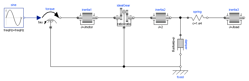
First create a Python script file and enter the usual imports:
import matplotlib.pyplot as plt
from pymodelica import compile_fmu
from pyfmi import load_fmu
Next, the model is compiled and loaded:
# Compile model
fmu_name = compile_fmu("Modelica.Mechanics.Rotational.Examples.First")
# Load model
model = load_fmu(fmu_name)
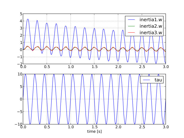
Notice that no file name, just an empty tuple, is provided to the function compile_fmu, since in this case the model that is compiled resides in the Modelica Standard Library. In the compilation process, the index reduction algorithm is invoked. Next, the model is simulated for 3 seconds:
# Load result file
res = model.simulate(final_time=3.)
Finally, the simulation results are retrieved and plotted:
w1 = res['inertia1.w']
w2 = res['inertia2.w']
w3 = res['inertia3.w']
tau = res['torque.tau']
t = res['time']
plt.figure(1)
plt.subplot(2,1,1)
plt.plot(t,w1,t,w2,t,w3)
plt.grid(True)
plt.legend(['inertia1.w','inertia2.w','inertia3.w'])
plt.subplot(2,1,2)
plt.plot(t,tau)
plt.grid(True)
plt.legend(['tau'])
plt.xlabel('time [s]')
plt.show()
You should now see a plot as shown below.
Simulation and parameter sweeps🔗
This example demonstrates how to run multiple simulations with different parameter values. Sweeping parameters is a useful technique for analysing model sensitivity with respect to uncertainty in physical parameters or initial conditions. Consider the following model of the Van der Pol oscillator:
model VDP
    // State start values
    parameter Real x1_0 = 0;
    parameter Real x2_0 = 1;

    // The states
    Real x1(start = x1_0);
    Real x2(start = x2_0);

    // The control signal
    input Real u;

equation
    der(x1) = (1 - x2^2) * x1 - x2 + u;
    der(x2) = x1;
end VDP;
Notice that the initial values of the states are parametrized by the parameters x1_0 and x2_0. Next, copy the Modelica code above into a file VDP.mo and save it in your working directory. Also, create a Python script file and name it vdp_pp.py. Start by copying the commands:
import numpy as N
import pylab as P
from pymodelica import compile_fmu
from pyfmi import load_fmu
into the Python file. Compile and load the model:
# Define model file name and class name
model_name = 'VDP'
mofile = 'VDP.mo'

# Compile model
fmu_name = compile_fmu(model_name,mofile)
Next, we define the initial conditions for which the parameter sweep will be done. The state x2 starts at 0, whereas the initial condition for x1 is swept between -3 and 3:
# Define initial conditions
N_points = 11
x1_0 = N.linspace(-3.,3.,N_points)
x2_0 = N.zeros(N_points)
In order to visualize the results of the simulations, we open a plot window:
fig = P.figure()
P.clf()
P.xlabel('x1')
P.ylabel('x2')
The actual parameter sweep is done by looping over the initial condition vectors and in each iteration set the parameter values into the model, simulate and plot:
for i in range(N_points):
# Load model
vdp = load_fmu(fmu_name)
# Set initial conditions in model
vdp.set('x1_0',x1_0[i])
vdp.set('x2_0',x2_0[i])
# Simulate
res = vdp.simulate(final_time=20)
# Get simulation result
x1=res['x1']
x2=res['x2']
# Plot simulation result in phase plane plot
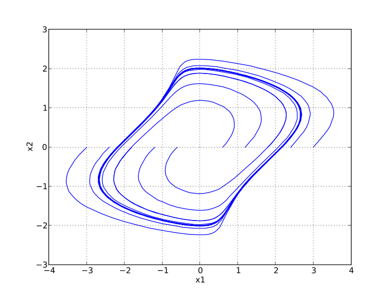
P.plot(x1, x2,'b')
P.grid()
P.show()
You should now see a plot similar to that in Figure 5.4
Simulation of an Engine model with inputs🔗
In this example, the model is larger than the previous one. It is a slightly modified version of the model EngineV6_analytic from the Multibody library in the Modelica Standard Library. The modification consists of a replaced load with a user-defined load. This has been done to be able to demonstrate how inputs are set from a Python script. In Figure 5.5 the model is shown.
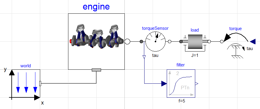
The Modelica code for the model is shown below, copy and save the code in a file named EngineV6.mo
model EngineV6_analytic_with_input
  output Real engineSpeed_rpm= Modelica.Units.SI.Conversions.to_rpm(load.w);
  output Real engineTorque = filter.u;
  output Real filteredEngineTorque = filter.y;

  input Real u;

  import Modelica.Mechanics.*;
  inner MultiBody.World world;
  MultiBody.Examples.Loops.Utilities.EngineV6_analytic engine(redeclare
     model Cylinder = MultiBody.Examples.Loops.Utilities.Cylinder_analytic_CAD);

  Rotational.Components.Inertia load(
    phi(start=0,fixed=true), w(start=10,fixed=true),
    stateSelect=StateSelect.always,J=1);
  Rotational.Sensors.TorqueSensor torqueSensor;
  Rotational.Sources.Torque torque;

  Modelica.Blocks.Continuous.CriticalDamping filter(
    n=2,initType=Modelica.Blocks.Types.Init.SteadyState,f=5);
equation
  torque.tau = u;

  connect(world.frame_b, engine.frame_a);
  connect(torque.flange, load.flange_b);
  connect(torqueSensor.flange_a, engine.flange_b);
  connect(torqueSensor.flange_b, load.flange_a);
  connect(torqueSensor.tau, filter.u);
  annotation (experiment(StopTime=1.01));
end EngineV6_analytic_with_input;
Now that the model has been defined, we create our Python script which will compile, simulate and visualize the result for us. Create a new text-file and start by copying the below commands into the file. The code will import the necessary methods and packages into Python.
from pymodelica import compile_fmu
from pyfmi import load_fmu
import pylab as P
Compiling the model is performed by invoking the compile_fmu method where the first argument is the name of the model and the second argument is where the model is located (which file). The method will create an FMU in the current directory and to simulate the FMU, we need to additionally load the created FMU into Python. This is done with the load_fmu method which takes the name of the FMU as input.
name = compile_fmu("EngineV6_analytic_with_input", "EngineV6.mo")
model = load_fmu(name)
So, now that we have compiled the model and loaded it into Python we are almost ready to simulate the model. First, we retrieve the simulation options and specify how many result points we want to receive after a simulation.
opts = model.simulate_options()
opts["ncp"] = 1000 #Specify that 1000 output points should be returned
A simulation is finally performed using the simulate method on the model and as we have changed the options, we need to additionally provide these options to the simulate method.
P.plot(res["time"],res["filteredEngineTorque"], label="Filtered Engine Torque")
P.show()
In Figure 5.6 the trajectories are shown for he engine torque and the engine speed utilizing subplots from Matplotlib.
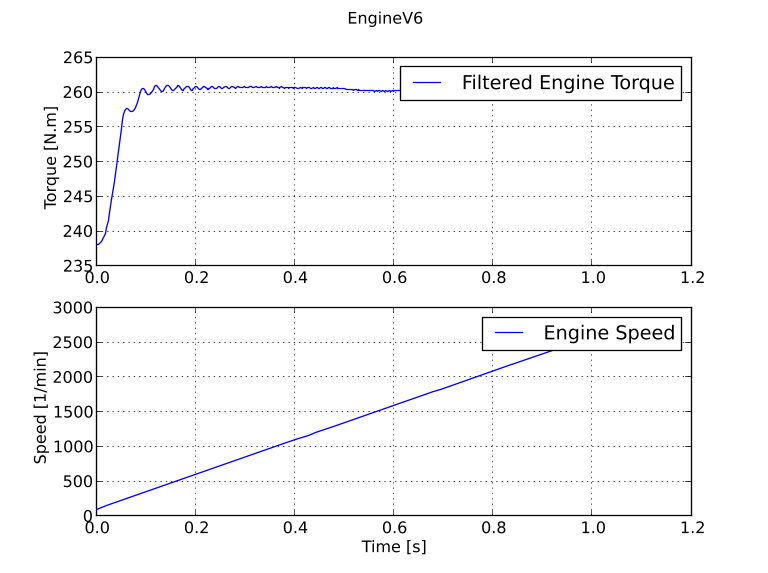
Above we have simulated the engine model and looked at the result, we have not however specified any load as input. Remember that the model we are looking at has a user-specified load. Now we will create a Python function that will act as our input. We create a function that depends on the time and returns the value for use as input.
def input_func(t):
    return -100.0*t
In order to use this input in the simulation, simply provide the name of the input variable and the function as the input argument to the simulate method, see below.
res = model.simulate(options=opts, input=("u",input_func))
Simulate the model again and look at the result and the impact of the input.
Large models contain an enormous amount of variables and by default, all of these variables are stored in the result. Storing the result takes time and for large models, the saving of the result may be responsible for the majority of the overall simulation time. Not all variables may be of interest, for example in our case, we are only interested in two variables so storing the other variables are not necessary. In the options dictionary there is a filter option which allows specifying which variables should be stored, so in our case, try the below filter and look at the impact on the simulation time.
opts["filter"] = ["filteredEngineTorque", "engineSpeed_rpm"]
Simulation using the native FMI interface🔗
This example shows how to use the native OCT FMI interface for the simulation of an FMU of version 2.0 for Model Exchange. For the procedure with version 1.0, refer to Functional Mock-up Interface for Model Exchange version 1.0.
The FMU that is to be simulated is the bouncing ball example from Qtronics FMU SDK . This example is written similarly to the example in the documentation of the 'Functional Mockup Interface for Model Exchange' version 2.0 https://www.fmi-standard.org/ The bouncing ball model is to be simulated using the explicit Euler method with event detection.
The example can also be found in the Python examples catalog in the OCT platform. There you can also find a similar example for simulation with a version 1.0 Model Exchange FMU.
The bouncing ball consists of two equations,

and one event function (also commonly called root function),

Where the ball bounces and loses some of its energy according to,

Here, h is the height, g the gravity, v the velocity and e a dimensionless parameter. The starting values are, h=1 and v=0 and for the parameters, e=0.7 and g = 9.81.
Implementation🔗
Start by importing the necessary modules,
import numpy as N
import pylab as P              # Used for plotting
from pyfmi.fmi import load_fmu # Used for loading the FMU
Next, the FMU is to be loaded and initialized
# Load the FMU by specifying the fmu together with the path.
bouncing_fmu = load_fmu('/path/to/FMU/bouncingBall.fmu')

Tstart = 0.5                                       # The start time.
Tend = 3.0                                         # The final simulation time.
# Initialize the model. Also sets all the start attributes defined in the XML file.

bouncing_fmu.setup_experiment(start_time = Tstart) # Set the start time to Tstart
bouncing_fmu.enter_initialization_mode()
bouncing_fmu.exit_initialization_mode()
he first line loads the FMU and connects the C-functions of the model to Python together with loading the information from the XML-file. The start time also needs to be specified by providing the argument start_time to setup_experiment. The model is also initialized, which must be done before the simulation is started.
Note that if the start time is not specified, FMUModelME2 tries to find the starting time in the XML-file structure 'default experiment' and if successful starts the simulation from that time. Also if the XML-file does not contain any information about the default experiment the simulation is started from time zero.
Next step is to do the event iteration and thereafter enter continuous time mode.
eInfo = bouncing_fmu.get_event_info()
eInfo.newDiscreteStatesNeeded = True
#Event iteration
while eInfo.newDiscreteStatesNeeded == True:
    bouncing_fmu.enter_event_mode()
    bouncing_fmu.event_update()
    eInfo = bouncing_fmu.get_event_info()

bouncing_fmu.enter_continuous_time_mode()
Then information about the first step is retrieved and stored for later use.
# Get Continuous States
x = bouncing_fmu.continuous_states
# Get the Nominal Values
x_nominal = bouncing_fmu.nominal_continuous_states
# Get the Event Indicators
event_ind = bouncing_fmu.get_event_indicators()

# Values for the solution
# Retrieve the valureferences for the values 'h' and 'v'
vref = [bouncing_fmu.get_variable_valueref('h')] + \
       [bouncing_fmu.get_variable_valueref('v')]
t_sol = [Tstart]
sol = [bouncing_fmu.get_real(vref)]
Here the continuous states together with the nominal values and the event indicators are stored to be used in the integration loop. In our case, the nominal values are all equal to one. This information is available in the XML-file. We also create lists that are used for storing the result. The final step before the integration is started is to define the step-size.
time = Tstart
Tnext = Tend # Used for time events
dt = 0.01 # Step-size
We are now ready to create our main integration loop where the solution is advanced using the explicit Euler method.
# Main integration loop.
while time < Tend and not bouncing_fmu.get_event_info().terminateSimulation:
    #Compute the derivative of the previous step f(x(n), t(n))
    dx = bouncing_fmu.get_derivatives()

    # Advance
    h = min(dt, Tnext-time)
    time = time + h

    # Set the time
    bouncing_fmu.time = time

    # Set the inputs at the current time (if any)
    # bouncing_fmu.set_real,set_integer,set_boolean,set_string (valueref, values)

    # Set the states at t = time (Perform the step using x(n+1)=x(n)+hf(x(n), t(n))
    x = x + h*dx
    bouncing_fmu.continuous_states = x
This is the integration loop for advancing the solution one step. The loop continues until the final time has been reached or if the FMU reported that the simulation is to be terminated. At the start of the loop, the derivatives of the continuous states are retrieved and then the simulation time is incremented by the step-size and set to the model. It could also be the case that the model depends on inputs that can be set using the set_(real/...) methods.
Note that only variables defined in the XML-file to be inputs can be set using the set_(real/...) methods according to the FMI specification.
The step is performed by calculating the new states (x+h*dx) and setting the values into the model. As our model, the bouncing ball also consists of event functions that needs to be monitored during the simulation, we have to check the indicators which are done below.
 # Get the event indicators at t = time
 event_ind_new = bouncing_fmu.get_event_indicators()

 # Inform the model about an accepted step and check for step events
 step_event = bouncing_fmu.completed_integrator_step()

 # Check for time and state events
 time_event = abs(time-Tnext) <= 1.e-10
 state_event = True if True in ((event_ind_new>0.0) != (event_ind>0.0)) else False
Events can be, time, state or step events. The time events are checked by continuously monitoring the current time and the next time event (Tnext). State events are checked against sign changes of the event functions. Step events are monitored in the FMU, in the method completed_integrator_step() and return True if any event handling is necessary. If an event has occurred, it needs to be handled, see below.
# Event handling
if step_event or time_event or state_event:
    bouncing_fmu.enter_event_mode()
    eInfo = bouncing_fmu.get_event_info()
    eInfo.newDiscreteStatesNeeded = True

    # Event iteration
    while eInfo.newDiscreteStatesNeeded:
        bouncing_fmu.event_update('0') # Stops at each event iteration
        eInfo = bouncing_fmu.get_event_info()
        # Retrieve solutions (if needed)
        if eInfo.newDiscreteStatesNeeded:
            # bouncing_fmu.get_real,get_integer,get_boolean,get_string(valueref)
            pass

    # Check if the event affected the state values and if so sets them
    if eInfo.valuesOfContinuousStatesChanged:
        x = bouncing_fmu.continuous_states

    # Get new nominal values.
    if eInfo.nominalsOfContinuousStatesChanged:
        atol = 0.01*rtol*bouncing_fmu.nominal_continuous_states

    # Check for new time event
    if eInfo.nextEventTimeDefined:
        Tnext = min(eInfo.nextEventTime, Tend)
    else:
        Tnext = Tend
    bouncing_fmu.enter_continuous_time_mode()
If an event occurred, we enter the iteration loop and the event mode where we loop until the solution of the new states has converged. During this iteration, we can also retrieve the intermediate values with the normal get methods. At this point, eInfo contains information about the changes made in the iteration. If the state values have changed, they are retrieved. If the state references have changed, meaning that the state variables no longer have the same meaning as before by pointing to another set of continuous variables in the model, for example in the case of dynamic state selection, new absolute tolerances are calculated with the new nominal values. Finally, the model is checked for a new time event and the continuous time mode is entered again.
event_ind = event_ind_new

# Retrieve solutions at t=time for outputs
# bouncing_fmu.get_real,get_integer,get_boolean,get_string (valueref)

t_sol += [time]
sol += [bouncing_fmu.get_real(vref)]
At the end of the loop, the solution is stored and the old event indicators are stored for use in the next loop.
After the loop has finished, by reaching the final time, we plot the simulation results
# Plot the height
P.figure(1)
P.plot(t_sol,N.array(sol)[:,0])
P.title(bouncing_fmu.get_name())
P.ylabel('Height (m)')
P.xlabel('Time (s)')
# Plot the velocity
P.figure(2)
P.plot(t_sol,N.array(sol)[:,1])
P.title(bouncing_fmu.get_name())
P.ylabel('Velocity (m/s)')
P.xlabel('Time (s)')
P.show()
and the figure below shows the results.
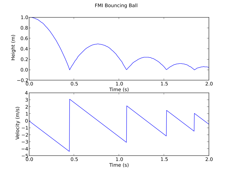
Simulation of Co-Simulation FMUs🔗
Simulation of a Co-Simulation FMU follows the same workflow as the simulation of a Model Exchange FMU. The model we would like to simulate is a model of a bouncing ball, the file bouncingBall.fmu is located in the examples folder in the OCT installation, pyfmi/examples/files/CS1.0/ for version 1.0 and pyfmi/examples/files/ CS2.0/ for version 2.0. The FMU is a Co-simulation FMU and to simulate it, we start by importing the necessary methods and packages into Python:
import pylab as P # For plotting
from pyfmi import load_fmu # For loading the FMU
Here, we have imported packages for plotting and the method load_fmu which takes as input an FMU and then determines the type and returns the appropriate class. Now, we need to load the FMU.
model = load_fmu('bouncingBall.fmu')
The model object can now be used to interact with the FMU, setting and getting values for instance. A simulation is performed by invoking the simulate method:
res = model.simulate(final_time=2.)
As a Co-Simulation FMU contains its own integrator, the method simulate calls this integrator. Finally, plotting the result is done as before:
# Retrieve the result for the variables
h_res = res['h']
_res = res['v']
t = res['time']
# Plot the solution
# Plot the height
fig = P.figure()
P.clf()
P.subplot(2,1,1)
P.plot(t, h_res)
P.ylabel('Height (m)')
P.xlabel('Time (s)')
# Plot the velocity
P.subplot(2,1,2)
P.plot(t, v_res)
P.ylabel('Velocity (m/s)')
P.xlabel('Time (s)')
P.suptitle('FMI Bouncing Ball')
P.show()
and the figure below shows the results
Cross-platform generation of FMUs🔗
While FMUs are generally specific to the platform they have been compiled on, OCT supports the generation of Windows FMUs on Ubuntu.
In this chapter, we describe how to generate a Windows FMU from Ubuntu (compiled with clang using libraries from Microsoft Visual C (MSVC) 2015). Both the MSVC runtime libraries and the Windows SDK are required.
Prerequisites and setup🔗
This feature requires that clang, version 19, and its cross-compilation toolchain is installed. Installation can be done as follows:
apt-get -y install wget lsb-release curl software-properties-common gnupg
wget https://apt.llvm.org/llvm.sh
chmod +x llvm.sh
./llvm.sh 19 all
Next, one needs to download the necessary MSVC libraries required for compilation. These can be downloaded using the tools and instructions at https://github.com/modelon-community/xwin.
OCT locates the MSVC libraries when compiling a model, by checking in the following order:
- The path specified in the compiler option target_platform_packages_directory.
- The environment variable OCT_CROSS_COMPILE_MSVC_DIR.
- The default location \<OCT_Install_folder>/lib/win64.
Modelica libraries with external code require compiled binaries compatible with the target platform, Windows, and that the external code is compiled using the Microsoft Visual C (MSVC) 2015 compiler. Note that libraries compiled with MSVC versions newer than 2015 could be compatible, since newer versions of MSVC strive to maintain backwards compatibility with older versions. But there is no guarantee that they are. Furthermore, the external code needs to be additionally compiled to work on the native platform, Ubuntu.
Limitations🔗
The following limitations apply to the cross-platform compilation of FMUs:
- OCT only supports cross-platform generation to Windows 64bit.
Example using the Python API🔗
The following example demonstrates how to compile a Windows FMU on Ubuntu, using the OCT Python API:
import os
from pymodelica import compile_fmu

msvc_dir_path = os.path.join('path', 'to', 'your', 'MSVC2015', 'libraries')
compiler_options = {'target_platform_packages_directory' : msvc_dir_path}
model = 'Modelica.Mechanics.Rotational.Examples.CoupledClutches'
fmu = compile_fmu(model, platform = 'win64', compiler_options = compiler_options)
Here, platform = 'win64' specifies that the target platform is Windows and the compiler option target_platform_packages_directory provides the compiler with the necessary MSVC libraries for a successful cross-platform compilation.
Dynamic Optimization in Python🔗
Introduction🔗
OCT supports the optimization of dynamic and steady state models. Many engineering problems can be cast as optimization problems, including optimal control, minimum time problems, optimal design, and model calibration. These different types of problems will be illustrated and it will be shown how they can be formulated and solved. The chapter starts with an introductory example in A first example and in Solving optimization problems, the details of how the optimization algorithms are invoked are explained. The following sections contain tutorial exercises that illustrate how to set up and solve different kinds of optimization problems.
When formulating optimization problems, models are expressed in the Modelica language, whereas optimization specifications are given in the Optimica extension which is described in Chapter 16 in OPTIMICA Compiler Toolkit User's guide. The tutorial exercises in this chapter assume that the reader is familiar with the basics of Modelica and Optimica.
A first example🔗
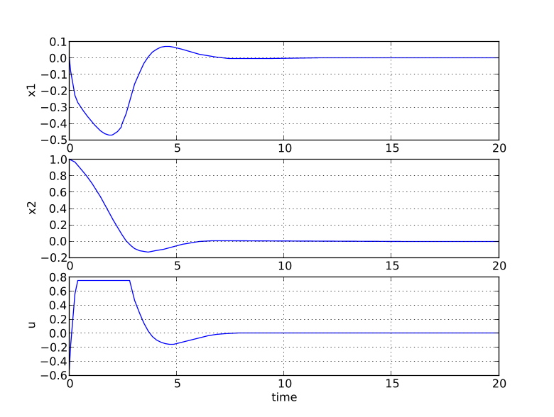
In this section, a simple optimal control problem will be solved. Consider the optimal control problem for the Van der Pol oscillator model:
optimization VDP_Opt (objectiveIntegrand = x1^2 + x2^2 + u^2,
                      startTime = 0,
                      finalTime = 20)

  // The states
  Real x1(start=0,fixed=true);
  Real x2(start=1,fixed=true);

  // The control signal
  input Real u;

equation
  der(x1) = (1 - x2^2) * x1 - x2 + u;
  der(x2) = x1;
constraint
  u<=0.75;
end VDP_Opt;
Create a new file named VDP_Opt.mop and save it in your working directory. Notice that this model contains both the dynamic system to be optimized and the optimization specification. This is possible since Optimica is an extension of Modelica and thereby supports also Modelica constructs such as variable declarations and equations. In most cases, however, Modelica models are stored separately from the Optimica specifications.
Next, create a Python script file and write (or copy-paste) the following commands:
# Import the function for transferring a model to CasADiInterface
from pyjmi import transfer_optimization_problem

# Import the plotting library
import matplotlib.pyplot as plt
Next, we transfer the model:
# Transfer the optimization problem to casadi
op = transfer_optimization_problem("VDP_Opt", "VDP_Opt.mop")
The function transfer_optimization_problem transfers the optimization problem into Python and expresses it's variables, equations, etc., using the automatic differentiation tool CasADi. This object represents the compiled model and is used to invoke the optimization algorithm:
res = op.optimize()
In this case, we use the default settings for the optimization algorithm. The result object can now be used to access the optimization result:
# Extract variable profiles
x1=res['x1']
x2=res['x2']
u=res['u']
t=res['time']
The variable trajectories are returned as NumPy arrays and can be used for further analysis of the optimization result or for visualization:
plt.figure(1)
plt.clf()
plt.subplot(311)
plt.plot(t,x1)
plt.grid()
plt.ylabel('x1')

plt.subplot(312)
plt.plot(t,x2)
plt.grid()
plt.ylabel('x2')

plt.subplot(313)
plt.plot(t,u)
plt.grid()
plt.ylabel('u')
plt.xlabel('time')
plt.show()
You should now see the optimization result as shown in Figure 6.1.
Solving optimization problems🔗
The first step when solving an optimization problem is to formulate a model and an optimization specification and then compile the model as described in the following sections in this chapter. There are currently two different optimization algorithms available in OCT, which are suitable for different classes of optimization problems.
• Dynamic optimization of DAEs using direct collocation with CasADi. This algorithm is the default algorithm for solving optimal control and parameter estimation problems. It is implemented in Python, uses CasADi for computing function derivatives and the nonlinear programming solver IPOPT for solving the resulting NLP. Use this method if your model is a DAE and does not contain discontinuities.
• Derivative free calibration and optimization of ODEs with FMUs. This algorithm solves parameter optimization and model calibration problems and is based on FMUs. The algorithm is implemented in Python and relies on a Nelder-Mead derivative free optimization algorithm. Use this method if your model is of large scale and has a modest number of parameters to calibrate and/or contains discontinuities or hybrid elements. Note that this algorithm is applicable to models which have been exported as FMUs also by other tools than OCT.
To illustrate how to solve optimization problems the Van der Pol problem presented above is used. First, the model is transferred into Python
op = transfer_optimization_problem("VDP_pack.VDP_Opt2", "VDP_Opt.mop")
All operations that can be performed on the model are available as methods of the op object and can be accessed by tab completion. Invoking an optimization algorithm is done by calling the method OptimizationProblem.optimize, which performs the following tasks:
• Sets up the selected algorithm with default or user-defined options
• Invokes the algorithm to find a numerical solution to the problem
• Writes the result to a file
• Returns a result object from which the solution can be retrieved
The interactive help for the optimize method is displayed by the command:
>>> help(op.optimize)
    Solve an optimization problem.
    Parameters::
        algorithm --
            The algorithm which will be used for the optimization is
            specified by passing the algorithm class name as string or
            class object in this argument. 'algorithm' can be any
            class which implements the abstract class AlgorithmBase
            (found in algorithm_drivers.py). In this way it is
            possible to write custom algorithms and to use them with this
            function.
            The following algorithms are available:
            - 'LocalDAECollocationAlg'. This algorithm is based on
              direct collocation on finite elements and the algorithm IPOPT
              is used to obtain a numerical solution to the problem.
            Default: 'LocalDAECollocationAlg'
        options --
            The options that should be used in the algorithm. The options
            documentation can be retrieved from an options object:

                >>> myModel = OptimizationProblem(...)
                >>> opts = myModel.optimize_options()
                >>> opts?

            Valid values are:
            - A dict that overrides some or all of the algorithm's default values.
              An empty dict will thus give all options with default values.
            - An Options object for the corresponding algorithm, e.g.
              LocalDAECollocationAlgOptions for LocalDAECollocationAlg.
            Default: Empty dict

    Returns::

        A result object, subclass of algorithm_drivers.ResultBase.
The optimize method can be invoked without any arguments, in which case the default optimization algorithm, with default options, is invoked:
res = vdp.optimize()
In the remainder of this Chapter the available algorithms are described in detail. Options for an algorithm can be set using the options argument to the optimize method. It is convenient to first obtain an options object in order to access the documentation and default option values. This is done by invoking the method optimize_options:
>>> help(op.optimize_options)
    Returns an instance of the optimize options class containing options
    default values. If called without argument then the options class for
    the default optimization algorithm will be returned.

    Parameters::
        algorithm --
            The algorithm for which the options class should be returned.
            Possible values are: 'LocalDAECollocationAlg'.
            Default: 'LocalDAECollocationAlg'

    Returns::

        Options class for the algorithm specified with default values.
The options object is essentially a Python dictionary and options are set simply by using standard dictionary syntax:
opts = vdp.optimize_options()
opts['n_e'] = 5
The optimization algorithm may then be invoked again with the new options:
res = vdp.optimize(options=opts)
Available options for each algorithm are documented in their respective sections in this Chapter.
The optimize method returns a result object containing the optimization result and some meta-information about the solution. The most common operation is to retrieve variable trajectories from the result object:
time = res['time']
x1 = res['x1']
Variable data is returned as NumPy arrays. The result object also contains references to the model that was optimized, the name of the result file that was written to disk, a solver object representing the optimization algorithm and an options object that was used when solving the optimization problem.
Scaling🔗
Many physical models contain variables with values that differ by several orders of magnitude. A typical example is thermodynamic models containing pressures, temperatures and mass flows. Such large differences in scales may have a severe deteriorating effect on the performance of numerical algorithms, and may in some cases even lead to the algorithm failing. In order to relieve the user from the burden of manually scaling variables, Modelica offers the nominal attribute, which can be used to automatically scale a model. Consider the Modelica variable declaration:
Real pressure(start=101.3e3, nominal=1e5);
Here, the nominal attribute is used to specify that the variable pressure takes on values that are on the order of 1e5. In order to use nominal attributes for scaling with CasADi-based algorithms, scaling is enabled by setting the algorithm option variable_scaling to True, and is enabled by default. When scaling is enabled, all variables with a set nominal attribute are then scaled by dividing the variable value by its nominal value, i.e., from an algorithm point of view, all variables should take on values close to one. Notice that variables typically vary during a simulation or optimization and that it is therefore not possible to obtain perfect scaling. In order to ensure that model equations are fulfilled, each occurrence of a variable is multiplied by its nominal value in equations. For example, the equation:
T = f(p)
is replaced by the equation
T_scaled*T_nom = f(p_scaled*p_nom)
when variable scaling is enabled.
The algorithm in Dynamic optimization of DAEs using direct collocation with CasADi also has support for providing trajectories (obtained by for example simulation) that are used for scaling. This means that it usually is not necessary to provide nominal values for all variables and that it is possible to use time-varying scaling factors.
For debugging purposes, it is sometimes useful to write a simulation/optimization/initialization result to file in scaled format, in order to detect if there are some variables that require additional scaling. The option write_scaled_result has been introduced as an option to initialize, simulate and optimize methods for this purpose.
Dynamic optimization of DAEs using direct collocation with CasADi🔗
Algorithm overview🔗
The direct collocation method described in this section can be used to solve dynamic optimization problems, including optimal control problems and parameter optimization problems. In the collocation method, the dynamic model variable profiles are approximated by piecewise polynomials. This method of approximating a differential equation corresponds to a fixed step implicit Runge-Kutta scheme, where the mesh defines the length of each step. Also, the number of collocation points in each element, or step, needs to be provided. This number corresponds to the stage order of the Runge-Kutta scheme. The selection of mesh is analogous to the choice of step length in a one-step algorithm for solving differential equations. Accordingly, the mesh needs to be fine-grained enough to ensure a sufficiently accurate approximation of the differential constraint. The nonlinear programming (NLP) solver IPOPT is used to solve the nonlinear program resulting from collocation. The needed first- and second-order derivatives are obtained using CasADi by algorithmic differentiation. For more details on the inner workings of the algorithm, see [Mag2015] and Chapter 3 in [Mag2016].
The NLP solver requires that the model equations are twice continuously differentiable with respect to all of the variables. This for example means that the model can not contain integer variables or if clauses depending on the states.
Optimization models are represented using the class OptimizationProblem, which can be instantiated using the transfer_optimization_problem method. An object containing all the options for the optimization algorithm can be retrieved from the object:
from pyjmi import transfer_optimization_problem
op = transfer_optimization_problem(class_name, optimica_file_path)
opts = op.optimize_options()
opts? # View the help text
After options have been set, the options object can be propagated to the optimize method, which solves the optimization problem:
res = op.optimize(options=opts)
The standard options for the algorithm are shown in Table 5. Additional documentation is available in the Python class documentation. The algorithm also has a lot of experimental options, which are not as well tested and some are intended for debugging purposes. These are shown in Table 6, and caution is advised when changing their default values.
| Options | Default | Description |
|---|---|---|
| n_e | 50 | Number of finite elements |
| hs | None | Element lengths. Possible values: None, iterable of floats and "free" None: The element lengths are uniformly distributed. iterable of floats: Component i of the iterable specifies the length of element i. The lengths must be normalized in the sense that the sum of all lengths must be equal to 1. "free": The element lengths become optimization variables and are optimized according to the algorithm option free_element_lengths_data. WARNING: The "free" option is very experimental and will not always give desirable results. |
| n_cp | 3 | Number of collocation points in each element. |
| expand_to_sx | "NLP" | Whether to expand the CasADi MX graphs to SX graphs. Possible values: "NLP", "DAE", "no". "NLP": The entire NLP graph is expanded into SX. This will lead to high evaluation speed and high memory consumption. "DAE": The DAE, objective and constraint graphs for the dynamic optimization problem expressions are expanded into SX, but the full NLP graph is an MX graph. This will lead to moderate evaluation speed and moderate memory consumption. "no": All constructed graphs are MX graphs. This will lead to low evaluation speed and low memory consumption. |
| init_traj | None | Variable trajectory data used for initialization of the NLP variables. |
| nominal_traj | None | Variable trajectory data used for scaling of the NLP variables. This option is only applicable if the variable scaling is enabled. |
| blocking_factors | None (not used) | Blocking factors are used to enforce piecewise constant inputs. The inputs may only change values at some of the element boundaries. The option is either None (disabled), given as an instance of pyjmi.optimization.casadi_collocation.BlockingFactors or as a list of blocking factors. If the options are a list of blocking factors, then each element in the list specifies the number of collocation elements for which all of the inputs must be constant. For example, if blocking_factors == [2, 2, 1], then the inputs will attain 3 different values (number of elements in the list), and it will change values between collocation element number 2 and 3 as well as numbers 4 and 5. The sum of all elements in the list must be the same as the number of collocation elements and the length of the list determines the number of separate values that the inputs may attain. See the documentation of the BlockingFactors class for how to use it. If blocking_factors is None, then the usual collocation polynomials are instead used to represent the controls. |
| external_data | None | Data used to penalize, constrain or eliminate certain variables. |
| delayed_feedback | None | If not *None*, should be a dict with mappings '*delayed_var*': ('*undelayed_var*', *delay_ne*). For each key-value pair, adds the constraint that the variable '*delayed_var*' equals the value of the variable '*undelayed_var*' delayed by *delay_ne* elements. The initial part of the trajectory for *'delayed_var'* is fixed to its initial guess given by the *init_traj* option or the *initialGuess* attribute. *'delayed_var'* will typically be an input. This is an experimental feature and is subject to change. |
| verbosity | 3 | Sets verbosity of algorithm output. 0 prints nothing, 3 prints everything. |
| IPOPT_options | IPOPT defaults | IPOPT options for solution of NLP. See IPOPT's documentation for available options |
| Options | Default | Description |
|---|---|---|
| free_element_lengths_data | None | Data used for optimizing the element lengths if they are free. Should be None when hs != "free". |
| discr | 'LGR' | Determines the collocation scheme used to discretize the problem. Possible values: "LG" and "LGR". "LG": Gauss collocation (Legendre-Gauss) "LGR": Radau collocation (Legendre-Gauss-Radau). |
| named_vars | False | If enabled, the solver will create a duplicated set of NLP variables which have names corresponding to the Modelica/Optimica variable names. Symbolic expressions of the NLP consisting of the named variables can then be obtained using the get_named_var_expr method of the collocator class. This option is only intended for investigative purposes. |
| init_dual | None | Dictionary containing vectors of the initial guess for NLP dual variables. Intended to be obtained as the solution to an optimization problem that has an identical structure, which is stored in the dual_opt attribute of the result object. The dictionary has two keys, 'g' and 'x', containing vectors of the corresponding dual variable initial guesses. Note that when using IPOPT, the option warm_start_init_point has to be activated for this option to have an effect. |
| variable_scaling | True | Whether to scale the variables according to their nominal values or the trajectories provided with the nominal_traj option. |
| equation_scaling | False | Whether to scale the equations in collocated NLP. Many NLP solvers default to scaling the equations, but if it is done through this option the resulting scaling can be inspected. |
| nominal_traj_mode | "_default_mode": "linear"} | Mode for computing scaling factors based on nominal trajectories. Four possible modes: "attribute": Timeinvariant, linear scaling based on Nominal attribute "linear": Time-invariant, linear scaling "affine": Timeinvariant, affine scaling "time-variant": Time-variant, linear scaling Option is a dictionary with variable names as keys and corresponding scaling modes as values. For all variables not occurring in the keys of the dictionary, the mode specified by the "_default_mode" entry will be used, which by default is "linear". |
| result_file_name | "" | Specifies the name of the file where the result is written. Setting this option to an empty string results in a default file name that is based on the name of the model class. |
| write_scaled_result | False | Return the scaled optimization result if set to True, otherwise return the unscaled optimization result. This option is only applicable when variable_scaling is enabled and is only intended for debugging. |
| print_condition_numbers | False | Prints the condition numbers of the Jacobian of the constraints and of the simplified KKT matrix at the initial and optimal points. Note that this is only feasible for very small problems. |
| result_mode | 'collocation_points' | Specifies the output format of the optimization result. Possible values: "collocation_points", "element_interpolation" and "mesh_points" "collocation_points": The optimization result is giv- en at the collocation points as well as the start and final time point. "element_interpolation": The values of the variable trajectories are calculated by evaluating the collocation polynomials. The algorithm option n_eval_points is used to specify the evaluation points within each finite element. "mesh_points": The optimization result is given at the mesh points. |
| n_eval_points | 20 | The number of evaluation points used in each element when the algorithm option result_mode is set to "element_interpolation". One evaluation point is placed at each element end-point (hence the option value must be at least 2) and the rest are distributed uniformly. |
| checkpoint | False | If checkpoint is set to True, transcribed NLP is built with packed MX functions. Instead of calling the DAE residual function, the collocation equation function, and the Lagrange term function n_e * n_cp times, the check point scheme builds an MXFunction evaluating n_cp collocation points at the same time, so that the packed MXFunction is called only n_e times. This approach improves code generation and it is expected to reduce memory usage for constructing and solving the NLP. |
| quadrature_constraint | True | Whether to use quadrature continuity constraints. This option is only applicable when using Gauss collocation. It is incompatible with eliminate_der_var set to True. True: Quadrature is used to get the values of the states at the mesh points. False: The Lagrange basis polynomials for the state collocation polynomials are evaluated to get the values of the states at the mesh points. |
| mutable_external_data | True | If true and the external_data option is used, the external data can be changed after discretization, e.g. during warm starting. |
| explicit_hessian | False | Explicitly construct the Lagrangian Hessian, rather than rely on CasADi to automatically generate it. This is only done to circumvent a bug in CasADi, see #4313, which rarely causes the automatic Hessian to be incorrect. |
| order | "defaults" | Order of variables and equations. Requires write_scaled_result! Possible values: "default", "reverse", and "random" |
The last standard option, IPOPT_options, serves as interface for setting options in IPOPT. To exemplify the usage of this interface, the maximum number of iterations in IPOPT can be set using the following syntax:
opts = model.optimize_options()
opts["IPOPT_options"]["max_iter"] = 10000
OCT's CasADi-based framework does not support the simulation and initialization of models. It is recommended to use PyFMI for these purposes instead.
Some statistics from the NLP solver can be obtained by issuing the command
res_opt.get_solver_statistics()
The return argument of this function can be found by using the interactive help:
help(res_opt.get_solver_statistics)
Get nonlinear programming solver statistics.
Returns::

    return_status --
    Return status from nonlinear programming solver.

    nbr_iter --
    Number of iterations.

    objective --
    Final value of objective function.

    total_exec_time --
    Execution time.
Reusing the same discretization for several optimization solutions🔗
When collocation is used to solve a dynamic optimization problem, the solution procedure is carried out in several steps:
• Discretize the dynamic optimization problem, which is formulated in continuous time. The result is a large and sparse nonlinear program (NLP). The discretization step depends on the options as provided to the optimize method.
• Solve the NLP.
• Postprocess the NLP solution to extract an approximate solution to the original dynamic optimization problem. Depending on the problem, discretization may account for a substantial amount of the total solution time, or even dominate it.
The same discretization can be reused for several solutions with different parameter values, but the same options. Discretization will be carried out each time the optimize method is called on the model. Instead of calling model.optimize(options=opts), a problem can be discretized using the prepare_optimization method:
solver = model.prepare_optimization(options=opts)
Alternatively, the solver can be retrieved from an existing optimization result, as solver = res.get_solver(). Manipulating the solver (e.g. setting parameters) may affect the original optimization problem object and vice versa.
The obtained solver object represents the discretized problem, and can be used to solve it using its own optimize method:
res = solver.optimize()
While options cannot be changed in general, parameter values, initial trajectories, external data, and NLP solver options can be changed on the solver object. Parameter values can be updated with
solver.set(parameter_name, value)
New initial trajectories can be set with
solver.set_init_traj(init_traj)
where init_traj has the same format as used with the init_traj option.
External data can be updated with
solver.set_external_variable_data(variable_name, data)
(unless the mutable_external_data option is turned off). variable_name should correspond to one of the variables used in the external_data option passed to prepare_optimization. data should be the new data, in the same format as variable data used in the external_data option. The kind of external data used for the variable (eliminated/constrained/quadratic penalty) is not changed.
Settings to the nonlinear solver can be changed with
solver.set_solver_option('IPOPT', name, value)
Warm starting🔗
The solver object obtained from prepare_optimization can also be used for warm starting, where an obtained optimization solution (including primal and dual variables) is used as the initial guess for a new optimization with new parameter values.
To reuse the solver's last obtained solution as initial guess for the next optimization, warm starting can be enabled with
solver.set_warm_start(True)
before calling solver.optimize(). This will reuse the last solution for the primal variables (unless solver.set_init_traj was called since the last solver.optimize) as well as the last solution for the dual variables.
When using the IPOPT solver with warm starting, several solver options typically also need to be set to see the benefits, e.g:
def set_warm_start_options(solver, push=1e-4, mu_init=1e-1):
    solver.set_solver_option('IPOPT', 'warm_start_init_point', 'yes')
    solver.set_solver_option('IPOPT', 'mu_init', mu_init)

    solver.set_solver_option('IPOPT', 'warm_start_bound_push', push)
    solver.set_solver_option('IPOPT', 'warm_start_mult_bound_push', push)
    solver.set_solver_option('IPOPT', 'warm_start_bound_frac', push)
    solver.set_solver_option('IPOPT', 'warm_start_slack_bound_frac', push)
    solver.set_solver_option('IPOPT', 'warm_start_slack_bound_push', push)

set_warm_start_options(solver)
Smaller values of the push and mu arguments will make the solver place more trust in that the sought solution is close to the initial guess, i e, the last solution.
Examples🔗
Optimal control🔗
his tutorial is based on the Hicks-Ray Continuously Stirred Tank Reactors (CSTR) system. The model was originally presented in [1]. The system has two states, the concentration, c, and the temperature, T. The control input to the system is the temperature, Tc, of the cooling flow in the reactor jacket. The chemical reaction in the reactor is exothermic, and also temperature dependent; high temperature results in a high reaction rate. The CSTR dynamics are given by:

This tutorial will cover the following topics:
• How to solve a DAE initialization problem. The initialization model has equations specifying that all derivatives should be identically zero, which implies that a stationary solution is obtained. Two stationary points, corresponding to different inputs, are computed. We call the stationary points A and B respectively. Point A corresponds to operating conditions where the reactor is cold and the reaction rate is low, whereas point B corresponds to a higher temperature where the reaction rate is high.
• An optimal control problem is solved where the objective is to transfer the state of the system from stationary point A to point B. The challenge is to ignite the reactor while avoiding uncontrolled temperature increases. It is also demonstrated how to set parameter and variable values in a model. More information about the simultaneous optimization algorithm can be found in OCT API documentation.
• The optimization result is saved to a file and then the important variables are plotted.
The Python commands in this tutorial may be copied and pasted directly into a Python shell, in some cases with minor modifications. Alternatively, you may copy the commands into a text file, e.g., cstr_casadi.py.
Start the tutorial by creating a working directory. In your installation, there is a directory named install, within the folder you find the filepath, python/pyjmi/examples/files/CSTR.mop. Copy this file to your working directory.
An online version of CSTR.mop is also available (depending on which browser you use, you may have to accept the site certificate by clicking through a few steps). If you choose to create a Python script file, save that as well to the working directory.
Compile and instantiate a model object🔗
The functions and classes used in the tutorial script need to be imported into the Python script. This is done by the following Python commands. Copy them and paste them either directly into your Python shell or, preferably, into your Python script file.
import numpy as N
import matplotlib.pyplot as plt
from pymodelica import compile_fmu
from pyfmi import load_fmu
from pyjmi import transfer_optimization_problem
To solve the initialization problem and simulate the model, we will first compile it as an FMU and load it in Python. These steps are described in more detail in Working with Models in Python.
# Compile the stationary initialization model into an FMU
init_fmu = compile_fmu("CSTR.CSTR_Init", "CSTR.mop")

# Load the FMU
init_model = load_fmu(init_fmu)
At this point, you may open the file CSTR.mop, containing the CSTR model and the static initialization model used in this section. Study the classes CSTR.CSTR and CSTR.CSTR_Init and make sure you understand the models. Before proceeding, have a look at the interactive help for one of the functions you used:
help(compile_fmu)
Solve the DAE initialization problem🔗
In the next step, we would like to specify the first operating point, A, by means of a constant input cooling temperature, and then solve the initialization problem assuming that all derivatives are zero.
# Set input for Stationary point A
Tc_0_A = 250
init_model.set('Tc', Tc_0_A)

# Solve the initialization problem using FMI
init_model.initialize()

# Store stationary point A
[c_0_A, T_0_A] = init_model.get(['c', 'T'])

# Print some data for stationary point A
print(' *** Stationary point A ***')
print('Tc = %f' % Tc_0_A)
print('c = %f' % c_0_A)
print('T = %f' % T_0_A)
Notice how the method set is used to set the value of the control input. The initialization algorithm is invoked by calling the method initialize, which returns a result object from which the initialization result can be accessed. The values of the states corresponding to point A can then be extracted from the result object. Look carefully at the printouts in the Python shell to see the stationary values. Display the help text for the initialize method and take a moment to look it through. The procedure is now repeated for operating point B:
# Set inputs for Stationary point B
init_model.reset() # reset the FMU so that we can initialize it again
Tc_0_B = 280
init_model.set('Tc', Tc_0_B)

# Solve the initialization problem using FMI
init_model.initialize()

# Store stationary point B
[c_0_B, T_0_B] = init_model.get(['c', 'T'])

# Print some data for stationary point B
print(' *** Stationary point B ***')
print('Tc = %f' % Tc_0_B)
print('c = %f' % c_0_B)
print('T = %f' % T_0_B)
We have now computed two stationary points for the system based on constant control inputs. In the next section, these will be used to set up an optimal control problem.
Solving an optimal control problem🔗
The optimal control problem we are about to solve is given by

and is expressed in Optimica format in the class CSTR.CSTR_Opt2 in the CSTR.mop file above. Have a look at this class and make sure that you understand how the optimization problem is formulated and what the objective is.
Direct collocation methods often require good initial guesses in order to ensure robust convergence. Also, if the problem is non-convex, initialization is even more critical. Since initial guesses are needed for all discretized variables along the optimization interval, simulation provides a convenient means to generate state and derivative profiles given an initial guess for the control input(s). It is then convenient to set up a dedicated model for the computation of initial trajectories. In the model CSTR.CSTR_Init_Optimization in the CSTR.mop file, a step input is applied to the system in order to obtain an initial guess. Notice that the variable names in the initialization model must match those in the optimal control model.
First, compile the model and set model parameters:
# Compile the optimization initialization model
init_sim_fmu = compile_fmu("CSTR.CSTR_Init_Optimization", "CSTR.mop")

# Load the model
init_sim_model = load_fmu(init_sim_fmu)

# Set initial and reference values
init_sim_model.set('cstr.c_init', c_0_A)
init_sim_model.set('cstr.T_init', T_0_A)
init_sim_model.set('c_ref', c_0_B)
init_sim_model.set('T_ref', T_0_B)
init_sim_model.set('Tc_ref', Tc_0_B)
Having initialized the model parameters, we can simulate the model using the simulate function.
# Simulate with constant input Tc
init_res = init_sim_model.simulate(start_time=0., final_time=150.)
The method simulate first computes consistent initial conditions and then simulates the model in the interval 0 to 150 seconds. Take a moment to read the interactive help for the simulate method.
The simulation result object is returned. Python dictionary access can be used to retrieve the variable trajectories.
# Extract variable profiles
t_init_sim = init_res['time']
c_init_sim = init_res['cstr.c']
T_init_sim = init_res['cstr.T']
Tc_init_sim = init_res['cstr.Tc']

# Plot the initial guess trajectories
plt.close(1)
plt.figure(1)
plt.subplot(3, 1, 1)
plt.plot(t_init_sim, c_init_sim)
plt.grid()
plt.ylabel('Concentration')
plt.title('Initial guess obtained by simulation')

plt.subplot(3, 1, 2)
plt.plot(t_init_sim, T_init_sim)
plt.grid()
plt.ylabel('Temperature')

plt.subplot(3, 1, 3)
plt.plot(t_init_sim, Tc_init_sim)
plt.grid()
plt.ylabel('Cooling temperature')
plt.xlabel('time')
plt.show()
Look at the plots and try to relate the trajectories to the optimal control problem. Why is this a good initial guess?
Once the initial guess is generated, we compile the optimal control problem:
# Compile and load optimization problem
op = transfer_optimization_problem("CSTR.CSTR_Opt2", "CSTR.mop")
We will now initialize the parameters of the model so that their values correspond to the optimization objective of transferring the system state from operating point A to operating point B. Accordingly, we set the parameters representing the initial values of the states to point A and the reference values in the cost function to point B:
# Set reference values
op.set('Tc_ref', Tc_0_B)
op.set('c_ref', float(c_0_B))
op.set('T_ref', float(T_0_B))

# Set initial values
op.set('cstr.c_init', float(c_0_A))
op.set('cstr.T_init', float(T_0_A))
We will also set some optimization options. In this case, we decrease the number of finite elements in the mesh from 50 to 19, to be able to illustrate that simulation and optimization might not give the exact same result. This is done by setting the corresponding option and providing it as an argument to the optimize method. We also lower the tolerance of IPOPT to get a more accurate result. We are now ready to solve the actual optimization problem. This is done by invoking the method optimize:
# Set options
opt_opts = op.optimize_options()
opt_opts['n_e'] = 19 # Number of elements
opt_opts['init_traj'] = init_res
opt_opts['nominal_traj'] = init_res
opt_opts['IPOPT_options']['tol'] = 1e-10
opt_opts['IPOPT_options']['linear_solver'] = "mumps""

# Solve the optimal control problem
res = op.optimize(options=opt_opts)
You should see the output of IPOPT in the Python shell as the algorithm iterates to find the optimal solution. IPOPT should terminate with a message like 'Optimal solution found' or 'Solved to acceptable level' in order for an optimum to have been found. The optimization result object is returned and the optimization data are stored in res.
We can now retrieve the trajectories of the variables that we intend to plot:
# Extract variable profiles
c_res = res['cstr.c']
T_res = res['cstr.T']
Tc_res = res['cstr.Tc']
time_res = res['time']
c_ref = res['c_ref']
T_ref = res['T_ref']
Tc_ref = res['Tc_ref']
Finally, we plot the result using the functions available in matplotlib:
# Plot the results
plt.close(2)
plt.figure(2)
plt.subplot(3, 1, 1)
plt.plot(time_res, c_res)
plt.plot(time_res, c_ref, '--')
plt.grid()
plt.ylabel('Concentration')
plt.title('Optimized trajectories')

plt.subplot(3, 1, 2)
plt.plot(time_res, T_res)
plt.plot(time_res, T_ref, '--')
plt.grid()
plt.ylabel('Temperature')

plt.subplot(3, 1, 3)
plt.plot(time_res, Tc_res)
plt.plot(time_res, Tc_ref, '--')
plt.grid()
plt.ylabel('Cooling temperature')
plt.xlabel('time')
plt.show()
You should now see the plot shown in Figure 6.2.
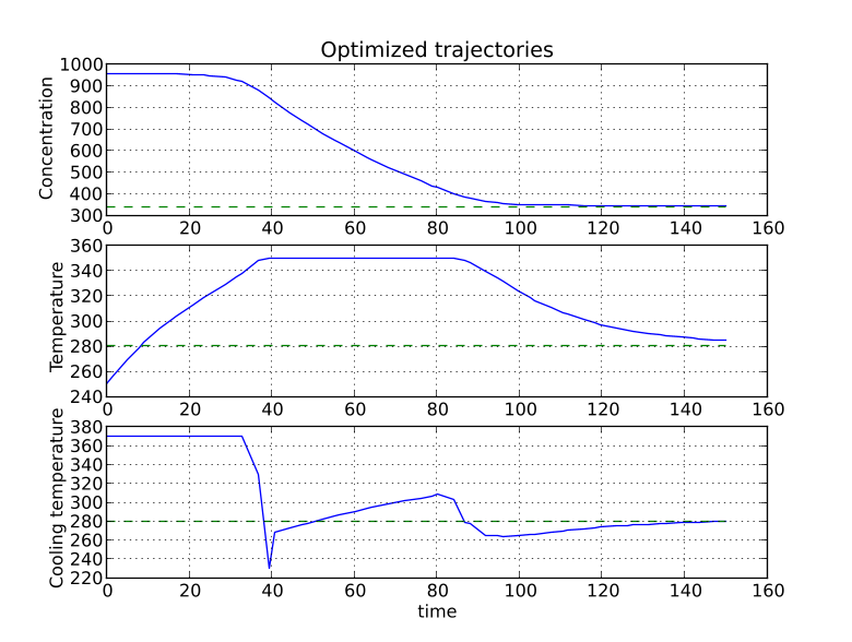
Take a minute to analyze the optimal profiles and to answer the following questions:
-
Why is the concentration high in the beginning of the interval?
-
Why is the input cooling temperature high in the beginning of the interval?
Verify optimal control solution🔗
Solving optimal control problems by means of direct collocation implies that the differential equation is approximated by a time-discrete counterpart. The accuracy of the solution is dependent on the method of collocation and the number of elements. In order to assess the accuracy of the discretization, we may simulate the system using the optimal control profile as input. With this approach, the state profiles are computed with high accuracy and the result may then be compared with the profiles resulting from optimization. Notice that this procedure does not verify the optimality of the resulting optimal control profiles, but only the accuracy of the discretization of the dynamics.
We start by compiling and loading the model used for simulation:
# Compile model
sim_fmu = compile_fmu("CSTR.CSTR", "CSTR.mop")

# Load model
sim_model = load_fmu(sim_fmu)
The solution obtained from the optimization is values at a finite number of time points, in this case the collocation points. The CasADi framework also supports obtaining all the collocation polynomials for all the input variables in the form of a function instead, which can be used during simulation for greater accuracy. We obtain it from the result object in the following manner.
# Get optimized input
(_, opt_input) = res.get_opt_input()
We specify the initial values and simulate using the optimal trajectory:
# Set initial values
sim_model.set('c_init', c_0_A)
sim_model.set('T_init', T_0_A)

# Simulate using optimized input
sim_opts = sim_model.simulate_options()
sim_opts['CVode_options']['rtol'] = 1e-6
sim_opts['CVode_options']['atol'] = 1e-8
res = sim_model.simulate(start_time=0., final_time=150.,
                         input=('Tc', opt_input), options=sim_opts)
Finally, we load the simulated data and plot it to compare it with the optimized trajectories:
# Extract variable profiles
c_sim=res['c']
T_sim=res['T']
Tc_sim=res['Tc']
time_sim = res['time']

# Plot the results
plt.figure(3)
plt.clf()
plt.subplot(311)
plt.plot(time_res,c_res,'--')
plt.plot(time_sim,c_sim)
plt.legend(('optimized','simulated'))
plt.grid()
plt.ylabel('Concentration')

plt.subplot(312)
plt.plot(time_res,T_res,'--')
plt.plot(time_sim,T_sim)
plt.legend(('optimized','simulated'))
plt.grid()
plt.ylabel('Temperature')

plt.subplot(313)
plt.plot(time_res,Tc_res,'--')
plt.plot(time_sim,Tc_sim)
plt.legend(('optimized','simulated'))
plt.grid()
plt.ylabel('Cooling temperature')
plt.xlabel('time')
plt.show()
You should now see the plot shown in Figure 6.3.
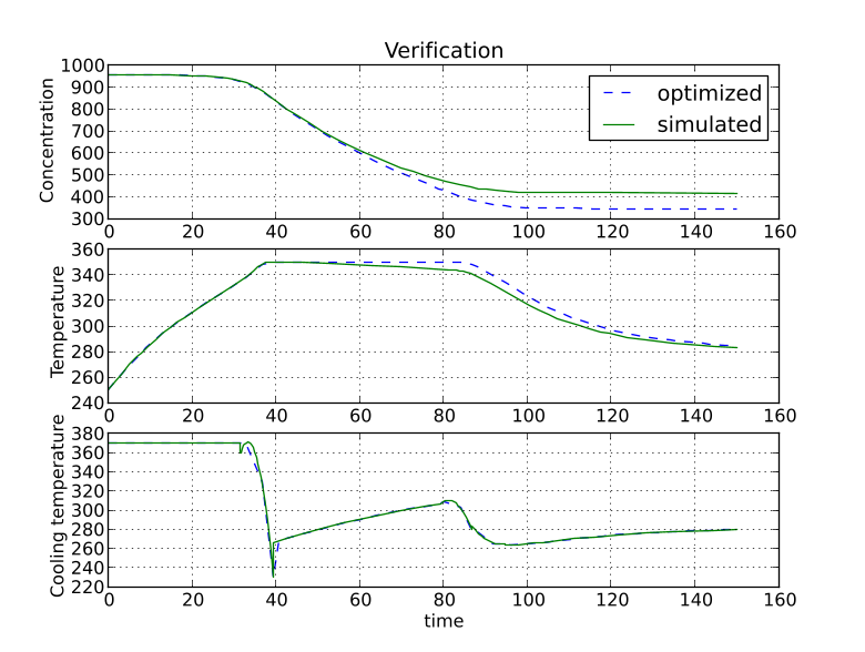
Discuss why the simulated trajectories differ from their optimized counterparts.
Exercises After completing the tutorial you may continue to modify the optimization problem and study the results.
-
Remove the constraint on cstr.T. What is then the maximum temperature?
-
Play around with weights in the cost function. What happens if you penalize the control variable with a larger weight? Do a parameter sweep for the control variable weight and plot the optimal profiles in the same figure.
-
Add terminal constraints (cstr.T(finalTime)=someParameter) for the states so that they are equal to point B at the end of the optimization interval. Now reduce the length of the optimization interval. How short can you make the interval?
-
Try varying the number of elements in the mesh and the number of collocation points in each interval.
References
[1] G.A. Hicks and W.H. Ray. Approximation Methods for Optimal Control Synthesis. Can. J. Chem. Eng., 40:522–529, 1971.
[2] Bieger, L., A. Cervantes, and A. Wächter (2002): "Advances in simultaneous strategies for dynamic optimization." Chemical Engineering Science, 57, pp. 575-593.
Minimum time problems🔗
Minimum time problems are dynamic optimization problems where not only the control inputs are optimized, but also the final time. Typically, elements of such problems include initial and terminal state constraints and an objective function where the transition time is minimized. The following example will be used to illustrate how minimum time problems are formulated in Optimica. We consider the optimization problem:


This problem is encoded in the following Optimica specification:
optimization VDP_Opt_Min_Time (objective = finalTime,
                               startTime = 0,
                               finalTime(free=true,min=0.2, initialGuess=1))

  // The states
  Real x1(start = 0,fixed=true);
  Real x2(start = 1,fixed=true);

  // The control signal
  input Real u(free=true,min=-1,max=1);

equation
  // Dynamic equations
  der(x1) = (1 - x2^2) * x1 - x2 + u;
  der(x2) = x1;
constraint
  // terminal constraints
  x1(finalTime)=0;
  x2(finalTime)=0;
end VDP_Opt_Min_Time;
Notice how the class attribute finalTime is set to be free in the optimization. The problem is solved by the following Python script:
# Import numerical libraries
import numpy as N
import matplotlib.pyplot as plt

# Import the OCT Python packages
from pymodelica import compile_fmu
from pyfmi import load_fmu
from pyjmi import transfer_optimization_problem

vdp = transfer_optimization_problem("VDP_Opt_Min_Time", "VDP_Opt_Min_Time.mop")
res = vdp.optimize()

# Extract variable profiles
x1=res['x1']
x2=res['x2']
u=res['u']
t=res['time']

# Plot
plt.figure(1)
plt.clf()
plt.subplot(311)
plt.plot(t,x1)
plt.grid()

plt.ylabel('x1')
plt.subplot(312)
plt.plot(t,x2)
plt.grid()
plt.ylabel('x2')

plt.subplot(313)
plt.plot(t,u,'x-')
plt.grid()
plt.ylabel('u')
plt.xlabel('time')
plt.show()
The resulting control and state profiles are shown in Figure 6.4. Notice the difference as compared to Figure 6.1, where the Van der Pol oscillator system is optimized using a quadratic objective function.
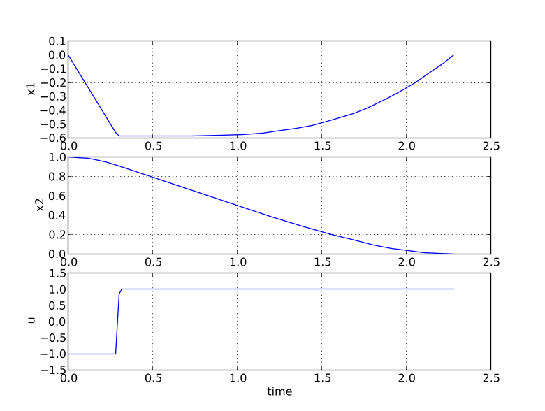
Optimization under delay constraints🔗
In some applications, it can be useful to solve dynamic optimization problems that include time delays in the model. Collocation-based optimization schemes are well suited to handle this kind of model, since the whole state trajectory is available at the same time. The direct collocation method using CasADi contains an experimental implementation of such delays, which we will describe with an example. Please note that the implementation of this feature is experimental and subject to change.
We consider the optimization problem

subject to the dynamics

and the boundary conditions

The effect of positive u1 is initially to increase x, but after a time delay of time tdelay , it comes back with twice the effect in the negative direction through u2 . We model everything except the delay constraint in the Optimica specification
optimization DelayTest(startTime = 0, finalTime = 1,
                       objectiveIntegrand = 4*x^2 + u1^2 + u2^2)
    input Real u1, u2;
    Real x(start = 1, fixed=true);
equation
    der(x) = u1 - 2*u2;
constraint
    x(finalTime) = 0;
end DelayTest;
The problem is then solved in the following Python script. Notice how the delay constraint is added using the delayed_feedback option, and the initial part is set using the initialGuess attribute:
# Import numerical libraries
import numpy as np
import matplotlib.pyplot as plt

# Import OCT Python packages
from pyjmi import transfer_optimization_problem

n_e = 20
delay_n_e = 5
horizon = 1.0
delay = horizon*delay_n_e/n_e

# Compile and load optimization problem
opt = transfer_optimization_problem("DelayTest", "DelayedFeedbackOpt.mop")

# Set value for u2(t) when t < delay
opt.getVariable('u2').setAttribute('initialGuess', 0.25)

# Set algorithm options
opts = opt.optimize_options()
opts['n_e'] = n_e

# Set delayed feedback from u1 to u2
opts['delayed_feedback'] = {'u2': ('u1', delay_n_e)}

# Optimize
res = opt.optimize(options=opts)

# Extract variable profiles
x_res = res['x']
u1_res = res['u1']
u2_res = res['u2']
time_res = res['time']

# Plot results
plt.plot(time_res, x_res, time_res, u1_res, time_res, u2_res)
plt.plot(time_res+delay, u1_res, '--')
plt.legend(('x', 'u1', 'u2', 'delay(u1)'))
plt.show()
The resulting control and state profiles are shown in Figure 6.5. Notice that x grows initially since u1 is set positive to exploit the greater control gain that appears delayed through u1 . At time 1 - tdelay , the delayed value of u1 ceases to influence x within the horizon, and u1 immediately switches sign to drive down to its final value.
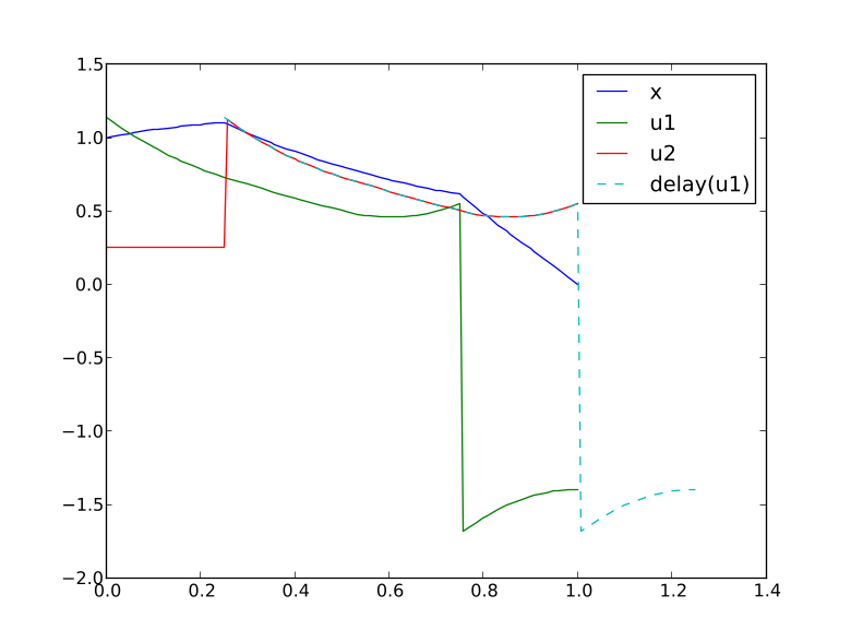
Parameter estimation🔗
In this tutorial it will be demonstrated how to solve parameter estimation problems. We consider a quadruple tank system depicted in Figure 6.6.
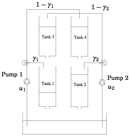
The dynamics of the system are given by the differential equations:

| Parameter name | Value | Unit |
|---|---|---|
| Ai | 4.9 | cm2 |
| ai | 0.03 | cm2 |
| ki | 0.56 | cm2 V-1 s-1 |
| γi | 0.3 | V cm2 |
The states of the model are the tank water levels x1, x2, x3, and x4. The control inputs, u1 and u2, are the flows generated by the two pumps.
The Modelica model for the system is located in QuadTankPack.mop. Download the file to your working directory and open it in a text editor. Locate the class QuadTankPack.QuadTank and make sure you understand the model. In particular, notice that all model variables and parameters are expressed in SI units.
Measurement data, available in qt_par_est_data.mat, has been logged in an identification experiment. Download also this file to your working directory.
Open a text file and name it qt_par_est_casadi.py. Then enter the imports:
import os
from collections import OrderedDict

from scipy.io.matlab.mio import loadmat
import matplotlib.pyplot as plt
import numpy as N

from pymodelica import compile_fmu
from pyfmi import load_fmu
from pyjmi import transfer_optimization_problem
from pyjmi.optimization.casadi_collocation import ExternalData
into the file. Next, we compile the model, which is used for simulation, and the optimization problem, which is used for estimating parameter values. We will take a closer look at the optimization formulation later, so do not worry about that one for the moment. The initial states for the experiment are stored in the optimization problem, which we propagate to the model for simulation.
# Compile and load FMU, which is used for simulation
model = load_fmu(compile_fmu('QuadTankPack.QuadTank', "QuadTankPack.mop"))

# Transfer problem to CasADi Interface, which is used for estimation
op = transfer_optimization_problem("QuadTankPack.QuadTank_ParEstCasADi",
                                   "QuadTankPack.mop")

# Set initial states in model, which are stored in the optimization problem
x_0_names = ['x1_0', 'x2_0', 'x3_0', 'x4_0']
x_0_values = op.get(x_0_names)
model.set(x_0_names, x_0_values)
Next, we enter code to open the data file, extract the measurement time series and plot the measurements:
# Load measurement data from file
data = loadmat("qt_par_est_data.mat", appendmat=False)
# Extract data series
t_meas = data['t'][6000::100, 0] - 60
y1_meas = data['y1_f'][6000::100, 0] / 100
y2_meas = data['y2_f'][6000::100, 0] / 100
y3_meas = data['y3_d'][6000::100, 0] / 100
y4_meas = data['y4_d'][6000::100, 0] / 100

u1 = data['u1_d'][6000::100, 0]
u2 = data['u2_d'][6000::100, 0]
# Plot measurements and inputs
plt.close(1)
plt.figure(1)
plt.subplot(2, 2, 1)
plt.plot(t_meas, y3_meas)
plt.title('x3')
plt.grid()
plt.subplot(2, 2, 2)
plt.plot(t_meas, y4_meas)
plt.title('x4')
plt.grid()
plt.subplot(2, 2, 3)
plt.plot(t_meas, y1_meas)
plt.title('x1')
plt.xlabel('t[s]')
plt.grid()
plt.subplot(2, 2, 4)
plt.plot(t_meas, y2_meas)
plt.title('x2')
plt.xlabel('t[s]')

plt.grid()
plt.close(2)
plt.figure(2)
plt.subplot(2, 1, 1)
plt.plot(t_meas, u1)
plt.title('u1')
plt.grid()
plt.subplot(2, 1, 2)
plt.plot(t_meas, u2)
plt.title('u2')
plt.xlabel('t[s]')
plt.grid()
plt.show()
You should now see two plots showing the measurement state profiles and the control input profiles similar to Figure 6.7 and Figure 6.8.
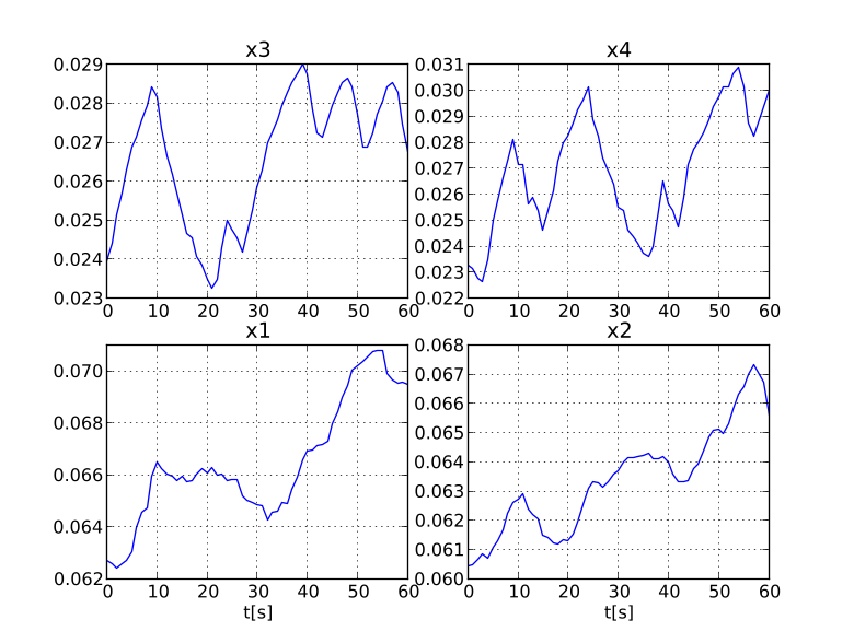
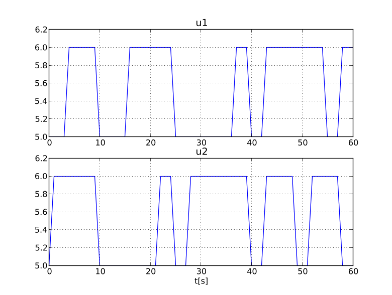
In order to evaluate the accuracy of nominal model parameter values, we simulate the model using the same initial state and inputs values as in the performed experiment used to obtain the measurement data. First, a matrix containing the input trajectories is created:
# Build input trajectory matrix for use in simulation
u = N.transpose(N.vstack([t_meas, u1, u2]))
Now, the model can be simulated:
# Simulate model response with nominal parameter values
res_sim = model.simulate(input=(['u1', 'u2'], u),
                         start_time=0., final_time=60.)
The simulation result can now be extracted:
# Load simulation result
x1_sim = res_sim['x1']
x2_sim = res_sim['x2']
x3_sim = res_sim['x3']
x4_sim = res_sim['x4']
t_sim = res_sim['time']
u1_sim = res_sim['u1']
u2_sim = res_sim['u2']
and then plotted:
# Plot simulation result
plt.figure(1)
plt.subplot(2, 2, 1)
plt.plot(t_sim, x3_sim)
plt.subplot(2, 2, 2)
plt.plot(t_sim, x4_sim)
plt.subplot(2, 2, 3)
plt.plot(t_sim, x1_sim)
plt.subplot(2, 2, 4)
plt.plot(t_sim, x2_sim)

plt.figure(2)
plt.subplot(2, 1, 1)
plt.plot(t_sim, u1_sim, 'r')
plt.subplot(2, 1, 2)
plt.plot(t_sim, u2_sim, 'r')
plt.show()
Figure 6.9 shows the result of the simulation.
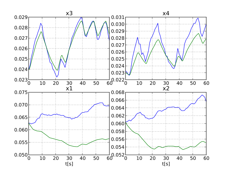
Here, the simulated profiles are given by the green curves. Clearly, there is a mismatch in the response, especially for the two lower tanks. Think about why the model does not match the data, i.e., which parameters may have wrong values.
The next step in solving a parameter estimation problem is to identify which parameters to tune. Typically, parameters that are not known precisely are selected. Also, the selected parameters need of course affect the mismatch between model response and data, when tuned. In a first attempt, we aim at decreasing the mismatch for the two lower tanks, and therefore we select the lower tank outflow areas, a1 and a2, as parameters to optimize. The Optimica specification for the estimation problem is contained in the class QuadTankPack.QuadTank_ParEstCasADi:
optimization QuadTank_ParEstCasADi(startTime=0, finalTime=60)

    extends QuadTank(x1(fixed=true), x1_0=0.06255,
                     x2(fixed=true), x2_0=0.06045,
                     x3(fixed=true), x3_0=0.02395,
                     x4(fixed=true), x4_0=0.02325,
                     a1(free=true, min=0, max=0.1e-4),
                     a2(free=true, min=0, max=0.1e-4));
end QuadTank_ParEstCasADi;
We have specified the time horizon to be one minute, which matches the length of the experiment, and that we want to estimate a1 and a2 by setting free=true for them. Unlike optimal control, the cost function is not specified using Optimica. This is instead specified from Python, using the ExternalData class and the code below.
# Create external data object for optimization
Q = N.diag([1., 1., 10., 10.])
data_x1 = N.vstack([t_meas, y1_meas])
data_x2 = N.vstack([t_meas, y2_meas])
data_u1 = N.vstack([t_meas, u1])
data_u2 = N.vstack([t_meas, u2])
quad_pen = OrderedDict()
quad_pen['x1'] = data_x1
quad_pen['x2'] = data_x2
quad_pen['u1'] = data_u1
quad_pen['u2'] = data_u2
external_data = ExternalData(Q=Q, quad_pen=quad_pen)
This will create an objective which is the integral of the squared difference between the measured profiles for x1 and x2 and the corresponding model profiles. We will also introduce corresponding penalties for the two input variables, which are left as optimization variables. It would also have been possible to eliminate the input variables from the estimation problem by using the eliminated parameter of ExternalData. See the documentation of ExternalData for how to do this. Finally, we use a square matrix Q to weight the different components of the objective. We choose larger weights for the inputs, as we have larger faith in those values.
We are now ready to solve the optimization problem. We first set some options, where we specify the number of elements (time-discretization grid), the external data, and also provide the simulation with the nominal parameter values as an initial guess for the solution, which is also used to scale the variables instead of the variables' nominal attributes (if they have any):
# Set optimization options and optimize
opts = op.optimize_options()
opts['n_e'] = 60 # Number of collocation elements
opts['external_data'] = external_data
opts['init_traj'] = res_sim
opts['nominal_traj'] = res_sim
res = op.optimize(options=opts) # Solve estimation problem
Now, let's extract the optimal values of the parameters a1 and a2 and print them to the console:
# Extract estimated values of parameters
a1_opt = res.initial("a1")
a2_opt = res.initial("a2")

# Print estimated parameter values
print('a1: ' + str(a1_opt*1e4) + 'cm^2')
print('a2: ' + str(a2_opt*1e4) + 'cm^2')
You should get an output similar to:
a1: 0.0266cm^2
a2: 0.0271cm^2
The estimated values are slightly smaller than the nominal values - think about why this may be the case. Also, note that the estimated values do not necessarily correspond to the physically true values. Rather, the parameter values are adjusted to compensate for all kinds of modeling errors in order to minimize the mismatch between model response and measurement data.
Next, we plot the optimized profiles:
# Load state profiles
x1_opt = res["x1"]
x2_opt = res["x2"]
x3_opt = res["x3"]
x4_opt = res["x4"]
u1_opt = res["u1"]
u2_opt = res["u2"]
t_opt = res["time"]

# Plot estimated trajectories
plt.figure(1)
plt.subplot(2, 2, 1)
plt.plot(t_opt, x3_opt, 'k')
plt.subplot(2, 2, 2)
plt.plot(t_opt, x4_opt, 'k')
plt.subplot(2, 2, 3)
plt.plot(t_opt, x1_opt, 'k')
plt.subplot(2, 2, 4)
plt.plot(t_opt, x2_opt, 'k')

plt.figure(2)
plt.subplot(2, 1, 1)
plt.plot(t_opt, u1_opt, 'k')
plt.subplot(2, 1, 2)
plt.plot(t_opt, u2_opt, 'k')
plt.show()
You will see the plot shown in Figure 6.10.
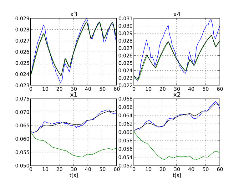
The profiles corresponding to the estimated values of a1 and a2 are shown in black curves. As can be seen, the match between the model response and the measurement data has been significantly improved. Is the behavior of the model consistent with the estimated parameter values?
Nevertheless, there is still a mismatch for the upper tanks, especially for tank 4. In order to improve the match, a second estimation problem may be formulated, where the parameters a1, a2, a3, a4 are free optimization variables, and where the squared errors of all four tank levels are penalized. Do this as an exercise!
Investigating optimization progress🔗
This section describes some tools that can be used to investigate the progress of the nonlinear programming solver on an optimization problem. This information can be useful when debugging convergence problems; some of it (e.g. dual variables) may also be useful to gain a better understanding of the properties of an optimization problem. To make sense of the information that can be retrieved, we first give an overview of the collocation procedure that transcribes the optimization problem into a Nonlinear Program (NLP).
Methods for inspecting progress are divided into low-level and high-level methods, where the low-level methods provide details of the underlying NLP while the high-level methods are oriented towards the optimization problem as seen in the model formulation.
All functionality related to the inspection of solver progress is exposed through the solver object as returned through the prepare_optimization method. If the optimization has been done through the optimize method instead, the solver can be obtained as in
res = op.optimize(options=opts)
solver = res.get_solver()
Collocation
To be able to solve a dynamic optimization problem, it is first discretized through collocation. Time is divided into elements (time intervals), and time-varying variables are approximated by a low-order polynomial over each element. Each polynomial piece is described by sample values at a number of collocation points (default 3) within the element. The result is that each time-varying variable in the model is instantiated into one NLP variable for each collocation point within each element. Some variables may also need to be instantiated at additional points, such as the initial point which is typically not a collocation point.
The equations in a model are divided into initial equations, DAE equations, path constraints and point constraints. These equations are also instantiated at different time points to become constraints in the NLP. Initial equations and point constraints are instantiated only once. DAE equations and path constraints are instantiated at collocation point of each element and possibly some additional points.
When using the methods described below, each model equation is referred to as a pair (eqtype, eqind). The string eqtype may be either 'initial', 'dae', 'path_eq', 'path_ineq', 'point_eq', or 'point_ineq'. The equation index eqind gives the index within the given equation type, and is a nonnegative integer less than the number of equations within the type. The symbolic model equations corresponding to given pairs (eqtype, eqind) can be retrieved through the get_equations method:
eq = solver.get_equations(eqtype, 0) # first equation of type eqtype
eqs = solver.get_equations(eqtype, [1,3]) # second and fourth equation
all_eqs = solver.get_equations(eqtype) # all equations of the given type
Apart from the model equations, collocation may also instantiate additional kinds of constraints, such as continuity constraints to enforce the continuity of states between elements and collocation constraints to prescribe the coupling between states and their derivatives. These constraints have their own eqtype strings. A list of all equation types that are used in a given model can be retrieved using
eqtypes = solver.get_constraint_types()
Inspecting residuals
Given a potential solution to the NLP, the residual of a constraint is a number that specifies how close it is to being satisfied. For equalities, the residual must be (close to) zero for the solution to be feasible. For inequalities, the residual must be in a specified range, typically nonpositive. The constraint violation is zero if the residual is within bounds, and gives the signed distance to the closest bound otherwise; for equality constraints, this is the same as the residual. Methods for returning residuals actually return the violation by default, but have an option to get the raw residual.
For a feasible solution, all violations are (almost) zero. If an optimization converges to an infeasible point or does not have time to converge to a feasible one then the residuals show which constraints the NLP solver was unable to satisfy. If one problematic constraint comes into conflict with a number of constraints, all of them will likely have nonzero violations. Residual values for a given equation type can be retrieved as a function of time through
r = solver.get_residuals(eqtype)
where r is an array of residuals of shape (n_timepoints, n_equations). There are also optional arguments: inds gives a subset of equation indices (e.g. inds=[0, 1]), point specifies whether to evaluate residuals at the optimization solution (point='opt', default) or the initial point (point='init'), and raw specifies whether to return constraint violations (raw=False, default) or raw residuals (raw=True).
The corresponding time points can be retrieved with
t, i, k = solver.get_constraint_points(eqtype)
where t, i, and k are vectors that give the time, element index, and collocation point index for each instantiation.
To get an overview of which residuals are the largest,
solver.get_residual_norms()
returns a list of equation types sorted by descending residual norm, and
solver.get_residual_norms(eqtype)
returns a list of equation indices of the given type sorted by residual norm.
By default, the methods above work with the unscaled residuals that result directly from collocation. If the equation_scaling option is turned on, the constraints will be rescaled before they are sent to the NLP solver. It might be of more interest to look at the size of the scaled residuals, since these are what the NLP solver will try to make small. The above methods can then be made to work with the scaled residuals instead of the unscaled by use of the scaled=True keyword argument. The residual scale factors can also be retrieved in analogy to solver.get_residuals through
scales = solver.get_residual_scales(eqtype)
and an overview of the residual scale factors (or inverse scale factors with inv=True) can be gained from
solver.get_residual_scale_norms()
Inspecting the constraint Jacobian
When solving the collocated NLP, the NLP solver typically has to evaluate the Jacobian of the constraint residual functions. Convergence problems can sometimes be related to numerical problems with the constraint Jacobian. In particular, IPOPT will never consider a potential solution if there are nonfinite (infinity or not-a-number) entries in the Jacobian. If the Jacobian has such entries at the initial guess, the optimizer will give up completely.
The constraint Jacobian comes from the NLP. As seen from the original model, it contains the derivatives of the model equations (and also e.g. the collocation equations) with respect to the model variables at different time points. If one or several problematic entries are found in the Jacobian, it is often helpful to know the model equation and variable that they correspond to. The set of (model equation, model variable) pairs that correspond to nonfinite entries in the constraint Jacobian can be printed with
solver.print_nonfinite_jacobian_entries()
or returned with
entries = solver.find_nonfinite_jacobian_entries()
There are also methods to allow to make more custom analyses of this kind. To instead list all Jacobian entries with an absolute value greater than 10, one can use
J = solver.get_nlp_jacobian() # Get the raw NLP constraint Jacobian as a (sparse)
 scipy.csc_matrix

# Find the indices of all entries with absolute value > 10
J.data = abs(J.data) > 10
c_inds, xx_inds = N.nonzero(J)

entries = solver.get_model_jacobian_entries(c_inds, xx_inds) # Map the indices to equations
 and variables in the model
solver.print_jacobian_entries(entries) # Print them
To get the Jacobian with residual scaling applied, use the scaled_residuals=True option.
Inspecting dual variables
Many NLP solvers (including IPOPT) produce a solution that consists of not only the primal variables (the actual NLP variables), but also one dual variable for each constraint in the NLP. Upon convergence, the value of each dual variable gives the change in the optimal objective per unit change in the residual. Thus, the dual variables can give an idea of which constraints are most hindering when it comes to achieving a lower objective value, however, they must be interpreted in relation to how much it might be possible to change any given constraint.
Dual variable values for a given equation type can be retrieved as a function of time through
d = solver.get_constraint_duals(eqtype)
in analogy to solver.get_residuals. To get constraint duals for the equation scaled problem, use the scaled=True keyword argument. Just as with get_residuals, the corresponding time points can be retrieved with
t, i, k = solver.get_constraint_points(eqtype)
Besides regular constraints, the NLP can also contain upper and lower bounds on variables. These will correspond to the Modelica min and max attributes for instantiated model variables. The dual variables for the bounds on a given model variable var can be retrieved as a function of time through
d = solver.get_bound_duals(var)
The corresponding time points can be retrieved with
t, i, k = solver.get_variable_points(var)
Inspecting low level information about NLP solver progress
The methods described above generally hide the actual collocated NLP and only require to work with model variables and equations, instantiated at different points. There also exist lower level methods that expose the NLP level information and its mapping to the original model more directly, and may be useful for more custom applications. These include
• get_nlp_variables, get_nlp_residuals, get_nlp_bound_duals, and get_nlp_constraint_duals to get raw vectors from the NLP solution.
• get_nlp_variable_bounds and get_nlp_residual_bounds to get the corresponding bounds used in the NLP.
• get_nlp_residual_scales to get the raw residual scale factors.
• get_nlp_variable_indices and get_nlp_constraint_indices to get mappings from model variables and equations to their NLP counterparts.
• get_point_time to get the times of collocation points (i, k).
• get_model_variables and get_model_constraints to map from NLP variables and constraints to the corresponding model variables and equations.
The low level constraint Jacobian methods get_nlp_jacobian, get_model_jacobian_entries, and the print_jacobian_entries method have already been covered in the section about jacobians above.
See the docstring for the respective method for more information.
Eliminating algebraic variables🔗
When the algorithm of this section is used, it is applied on the full DAE, meaning that all of the algebraic variables and equations are exposed to the numerical discretization and need to be solved by the NLP solver. It is often beneficial to instead solve some of these algebraic equations in a symbolic pre-processing step. This subsection describes how this can be done.
OCT has two different frameworks for performing such eliminations. The first one is not described in this User's Guide, but an example demonstrating its use can be found in pyjmi.examples.ccpp_elimination. It is implemented as a part of CasADi Interface, whereas the second framework, which is the focus of this subsection, is implemented in Python. The elimination framework in CasADi Interface has faster pre-processing, but has limitations regarding what kind of algebraic variables it can eliminate and also lacks important features such as tearing and sparsity preservation. For more details on the inner workings of the Python-based framework, see Chapter 4 in [Mag2016].
Basic use🔗
To leave everything in the hands of the framework, simply transfer an optimization problem as per usual and use the following Python code snippet.
from pyjmi.symbolic_elimination import BLTOptimizationProblem, EliminationOptions
op = transfer_optimization_problem(class_name, file_name) # Regular compilation
op = BLTOptimizationProblem(op) # Symbolically eliminate algebraic variables
You can then proceed as usual. There is however one caveat. The min and max attributes of eliminated algebraic variables will not be respected. If this is undesired, these bounds should either be converted into constraints (not recommended), or the corresponding variables should be marked as ineliminable as described in Small example.
Small example🔗
To demonstrate the use and effects of the framework, we consider the example pyjmi.examples.elimination_example. Note that this example is intended to be pedagogical, rather than showing the performance gains of the techniques. For a real-world example where the framework offers significant performance gains, see pyjmi.examples.ccpp_sym_elim, where the solution time is reduced by a factor of 5. The following artificial Modelica and Optimica code is used in this example.
optimization EliminationExample(finalTime=4,
                                objectiveIntegrand=(x1-0.647)^2+x2^2+(u-0.0595)^2+(y1-0.289)^2)
    Real x1(start=1, fixed=true);
    Real x2(start=1, fixed=true);
    Real y1(start=0.3, max=0.41);
    Real y2(start=1);
    Real y3(start=1);
    Real y4(start=1);
    Real y5(start=1);
    input Real u;
equation
    der(x1) = x2;
    der(x2) + y1 + y2 - y3 = u;
    x1*y3 + y2 - sqrt(x1) - 2 = 0;
    2*y1*y2*y4 - sqrt(x1) = 0;
    y1*y4 + sqrt(y3) - x1 - y4 = u;
    y4 - sqrt(y5) = 0;
    y5^2 - x1 = 0;
end EliminationExample;
We start as usual by transferring the optimization problem to CasADi Interface.
op = transfer_optimization_problem("EliminationExample", file_path, compiler_options={})
Next we prepare the symbolic elimination. An important part of this is the manual selection of algebraic variables that are not allowed to be eliminated. In general, it is recommended to not eliminate the following variables:
• Variables with potentially active bounds (min or max attributes). When variables are eliminated, their min and max attributes are neglected. This is because many Modelica variables have min and max attributes that are not intended to constrain the optimization solution. Preserving these bounds during elimination is highly inefficient. Since there is no way for the toolchain to know which variables may be actively constrained by their min and max attributes, it is up to the user to provide the names of these variables.
• Variables that occur in the objective or constraints. Marking these variables as ineliminable is less important, but can yield performance improvements.
• Variables that lead to numerically unstable pivots. When employing tearing, one runs the risk of causing numerically unstable computations. This is difficult to predict, but experienced users may know that certain variables should be selected for tearing to prevent instability, which can be achieved by marking them as ineliminable, which does not require a corresponding tearing residual to be chosen. Further details on manual tearing is described in Tearing.
In our small example, the only thing we have to worry about is y1, which has an upper bound. To mark y1 as ineliminable, we use the following code.
elim_opts = EliminationOptions()
elim_opts['ineliminable'] = ['y1'] # List of variable names
The elim_opts dictionary object is used to set any other elimination options, which are described in Available options. For now, we just enable the option to make a plot of the block-lower triangular (BLT) decomposition of the DAE incidence matrix, which gives insight regarding the performed eliminations (see [Mag2016]).
elim_opts['draw_blt'] = True
elim_opts['draw_blt_strings'] = True
Now we are ready to symbolically transform the optimization problem.
op = BLTOptimizationProblem(op, elim_opts)
This prints the following simple problem statistics.
System has 5 algebraic variables before elimination and 4 after.
The three largest BLT blocks have sizes 3, 1, and 1.
Since we enable the BLT drawing, we also get the following plot.
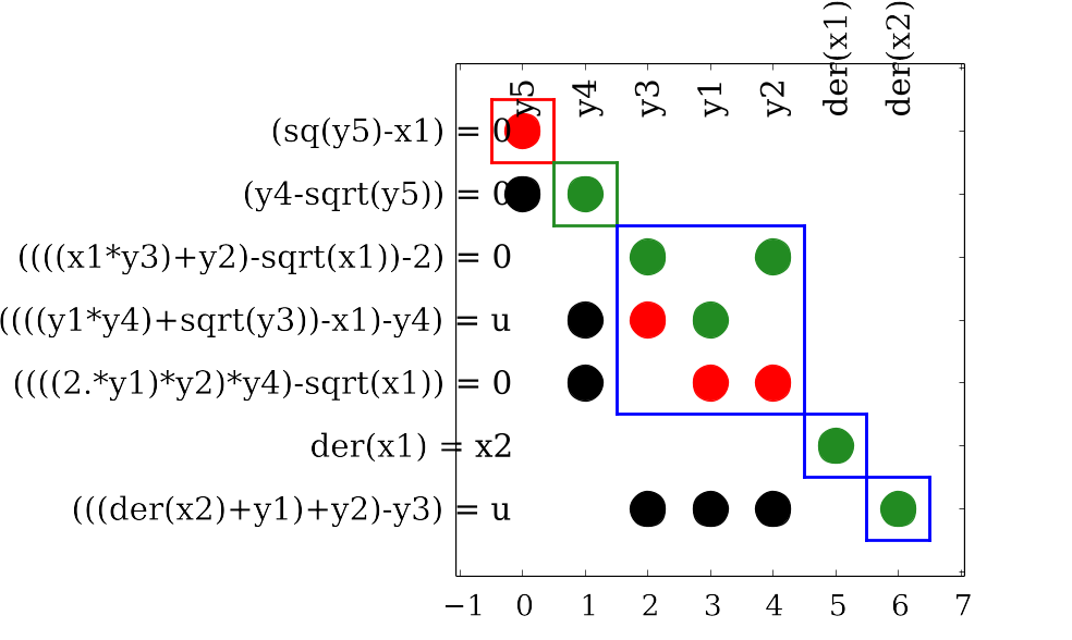
The only variable we were able to eliminate was y4. For details on what all the colors mean in the figure, see The many colors of symbolic elimination.
The many colors of symbolic elimination🔗
In the plots generated by enabling the option draw_blt, linear (with respect to the block variables) incidences are marked by green dots, and nonlinear incidences are marked by red dots. There is no distinction made between linear and nonlinear incidences outside of the diagonal blocks. Hence, such incidences are marked by black dots. Torn blocks are marked by red edges. Variables, and their respective matched equations, that have been user-specified as actively bounded (and hence are not eliminated) are marked by orange edges. State variable derivatives (which are not eliminated) and their respective matched equations are marked by blue edges. Blue edges are also used to mark non-scalar blocks that have not been torn. Variable–equation pairs along the diagonal that are not sparsity preserving are marked by yellow edges. The remaining variable–equation pairs along the diagonal are the ones used for elimination, which are marked by green edges.
Tearing🔗
By default, tearing is not used in the elimination. The use of tearing enables the elimination of variables in algebraic loops. In this example, we can also eliminate y2 through tearing. Tearing can either be done automatically or manually. Manual tearing is performed on the OptimizationProblem object, prior to symbolic transformation. To eliminate y2, we select the other variables in the algebraic loop for y2—that is, y3 and y1—as tearing variables as follows.
op.getVariable('y1').setTearing(True)
op.getVariable('y3').setTearing(True)
We also have to select tearing residuals. This is less convenient, as there is no straightforward way to identify an equation. We can either manually inspect the equations obtained from op.getDaeEquations(), or search through the string representations of all of them. We will adopt the second approach.
for eq in op_manual.getDaeEquations():
    eq_string = eq.getResidual().repr()
    if 'y1)*y2)*y4)' in eq_string or 'y1*y4' in eq_string:
        eq.setTearing(True)
Once the tearing selection is finished, the symbolic transformation can be performed as before by instantiating BLTOptimizationProblem.
For this example, we can get the same result by automatic tearing, which is enabled during compilation. We previously used compiler_options={}. By instead using
compiler_options = {'equation_sorting': True, 'automatic_tearing': True}
tearing will be performed automatically. This will mark the same variables and equations as tearing variables as we just did manually. Hence, it may be a good idea to first perform tearing automatically and then make any needed changes manually, rather than doing manual tearing from scratch. Automatic tearing will yield satisfactory performance for most problems, so manual tearing is only recommended for experts. For this example, we can also eliminate y1 through manual tearing, but since we have a bound on y1, this is not recommended anyway.
Available options🔗
The standard elimination options are listed below. All of these have been explained in the above subsections, except for the last two related to sparsity preservation. A higher density tolerance will allow for the elimination of more algebraic variables, but the resulting DAE will be dense. This parameter thus allows a trade-off between the sparsity and dimension of the DAE, both of which affect the performance of the optimization.
| Option | Default | Description |
|---|---|---|
| draw_blt | False | Whether to plot the BLT form. |
| draw_blt_strings | False | Whether to annotate plot of the BLT form with strings for variables and equations. |
| tearing | True | Whether to tear algebraic loops. |
| ineliminable | [] | List of names of variables that should not be eliminated. Particularly useful for variables with bounds. |
| dense_measure | 'lmfi' | Density measure for controlling density in causalized system. Possible values: ['lmfi', 'Markowitz']. Markowitz uses the Markowitz criterion and lmfi uses local minimum fill-in to estimate density. |
| dense_tol | 15 | Tolerance for controlling density in causalized system. Possible values: [-inf, inf] |
The below table lists the experimental and debugging elimination options, which should not be used by the typical user.
| Option | Default | Description |
|---|---|---|
| plots | False | Whether to plot intermediate results for matching and component computation. |
| solve_blocks | False | Whether to factorize coefficient matrices in non-scalar, linear blocks. |
| solve_torn_linear_blocks | False | Whether to solve causalized equations in torn blocks, rather than doing forward substitution as for nonlinear blocks. |
| inline | True | Whether to inline function calls (such as creation of linear systems). |
| linear_solver | "symbolicqr" | Which linear solver to use. See http:// casadi.sourceforge.net/api/html/d8/d6a/ classcasadi_1_1LinearSolver.html for possibilities |
| closed_form | False | Whether to create a closed form expression for residuals and solutions. Disables computations. |
| inline_solved | False | Whether to inline solved expressions in the closed form expressions (only applicable if closed_form == True). |
Derivative-Free Model Calibration of FMUs🔗
This tutorial demonstrates how to solve a model calibration problem using an algorithm that can be applied to Functional Mock-up Units. The model to be calibrated is the Furuta pendulum shown in Figure 6.12. The Furuta pendulum consists of an arm rotating in the horizontal plane and a pendulum which is free to rotate in the vertical plane. The construction has two degrees of freedom, the angle of the arm, φ, and the angle of the pendulum, θ . Copy the file \(JMODELICA_HOME/Python/pyjmi/examples/files/FMUs/Furuta*.fmu to your working directory. Note that the Furuta.fmu file is currently only supported on Windows. Measurement data for φ and θ is available in the file *\)JMODELICA_HOME/Python/pyjmi/examples/files/FurutaData.mat. Copy this file to your working directory as well. These measurements will be used for the calibration. Open a text file, name it furuta_par_est.py and enter the following imports:
from scipy.io.matlab.mio import loadmat
import matplotlib.pyplot as plt
import numpy as N
from pyfmi import load_fmu
from pyjmi.optimization import dfo
Then, enter code for opening the data file and extracting the measurement time series:
# Load measurement data from file
data = loadmat('FurutaData.mat',appendmat=False)
# Extract data series
t_meas = data['time'][:,0]
phi_meas = data['phi'][:,0]
theta_meas = data['theta'][:,0]
Now, plot the measurements:
# Plot measurements
plt.figure (1)
plt.clf()
plt.subplot(2,1,1)
plt.plot(t_meas,theta_meas,label='Measurements')
plt.title('theta [rad]')
plt.legend(loc=1)
plt.grid ()
plt.subplot(2,1,2)
plt.plot(t_meas,phi_meas,label='Measurements')
plt.title('phi [rad]')
plt.legend(loc=1)
plt.grid ()
plt.show ()
This code should generate Figure 6.13 showing the measurements of θ and φ.
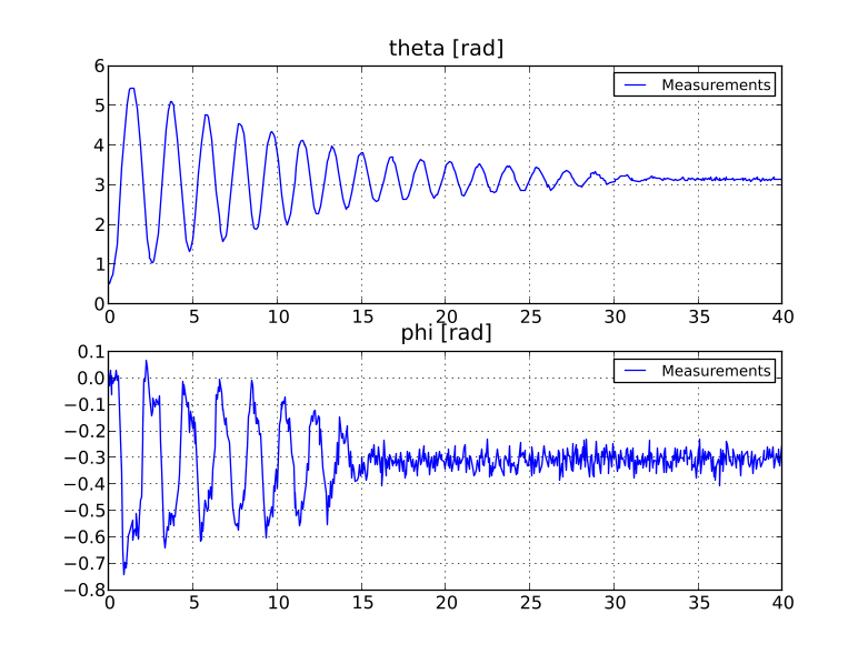
To investigate the accuracy of the nominal parameter values in the model, we shall now simulate the model:
# Load model
model = load_fmu("Furuta.fmu")
# Simulate model response with nominal parameters
res = model.simulate(start_time=0.,final_time=40)
# Load simulation result
phi_sim = res['armJoint.phi']
theta_sim = res['pendulumJoint.phi']
t_sim = res['time']
Then, we plot the simulation result:
# Plot simulation result
plt.figure (1)
plt.subplot(2,1,1)
plt.plot(t_sim,theta_sim,'--',label='Simulation nominal parameters')
plt.legend(loc=1)
plt.subplot(2,1,2)
plt.plot(t_sim,phi_sim,'--',label='Simulation nominal parameters')
plt.xlabel('t [s]')
plt.legend(loc=1)
plt.show ()
Figure 6.14 shows the simulation result together with the measurements.
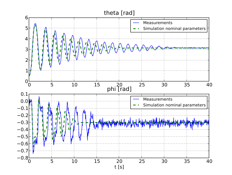
As can be seen, the simulation result does not quite agree with the measurements. We shall now attempt to calibrate the model by estimating the two following model parameters:
• carm: arm friction coefficient (nominal value 0.012)
• cpend: pendulum friction coefficient (nominal value 0.002)
The calibration will be performed using the Nelder-Mead simplex optimization algorithm. The objective function, i.e. the function to be minimized, is defined as:
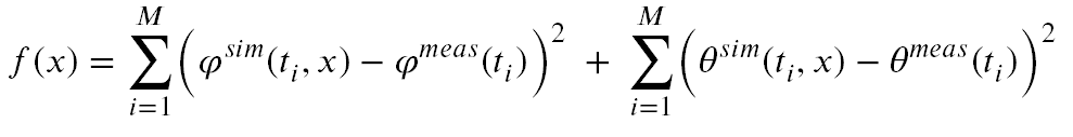
where ti, i = 1,2,...,M, are the measurement time points and [carm , cpend ]T is the parameter vector.φmeas and θmeas are the measurements of φ and θ, respectively, and φsim and θsim are the corresponding simulation results. Now, add code defining a starting point for the algorithm (use the nominal parameter values) as well as lower and upper bounds for the parameters:
# Choose starting point
x0 = N.array([0.012,0.002])*1e3
# Choose lower and upper bounds (optional)
lb = N.zeros (2)
ub = (x0 + 1e-2)*1e3
Note that the values are scaled with a factor 103. This is done to get a more appropriate variable size for the algorithm to work with. After the optimization is done, the obtained result is scaled back again. In this calibration problem, we shall use multiprocessing, i.e., parallel execution of multiple processes. All objective function evaluations in the optimization algorithm will be performed in separate processes in order to save memory and time. To be able to do this we need to define the objective function in a separate Python file and provide the optimization algorithm with the file name. Open a new text file, name it furuta_cost.py and enter the following imports:
from pyfmi import load_fmu
from pyjmi.optimization import dfo
from scipy.io.matlab.mio import loadmat
import numpy as N
Then, enter code for opening the data file and extracting the measurement time series:
# Load measurement data from file
data = loadmat('FurutaData.mat',appendmat=False)
# Extract data series
t_meas = data['time'][:,0]
phi_meas = data['phi'][:,0]
theta_meas = data['theta'][:,0]
Next, define the objective function, it is important that the objective function has the same name as the file it is defined in (except for .py):
# Define the objective function
def furuta_cost(x):
    # Scale down the inputs x since they are scaled up
    # versions of the parameters (x = 1e3*[param1,param2])
    armFrictionCoefficient = x[0]/1e3
    pendulumFrictionCoefficient = x[1]/1e3
    # Load model
    model = load_fmu('../Furuta.fmu')
    # Set new parameter values into the model
    model.set('armFriction',armFrictionCoefficient)
    model.set('pendulumFriction',pendulumFrictionCoefficient)
    # Simulate model response with new parameter values
    res = model.simulate(start_time=0.,final_time=40)
    # Load simulation result
    phi_sim = res['armJoint.phi']
    theta_sim = res['pendulumJoint.phi']
    t_sim = res['time']
    # Evaluate the objective function
    y_meas = N.vstack((phi_meas ,theta_meas))
    y_sim = N.vstack((phi_sim,theta_sim))
    obj = dfo.quad_err(t_meas,y_meas,t_sim,y_sim)
    return obj
This function will later be evaluated in temporary sub-directories to your working directory which is why the string '../' is added to the FMU name, it means that the FMU is located in the parent directory. The Python function dfo.quad_err evaluates the objective function. Now we can finally perform the actual calibration. Solve the optimization problem by calling the Python function dfo.fmin in the file named furuta_par_est.py:
# Solve the problem using the Nelder-Mead simplex algorithm
x_opt,f_opt,nbr_iters,nbr_fevals,solve_time = dfo.fmin("furuta_cost.py",
xstart=x0,lb=lb,ub=ub,alg=1,nbr_cores=4,x_tol=1e-3,f_tol=1e-2)
The input argument alg specifies which algorithm to be used, alg=1 means that the Nelder-Mead simplex algorithm is used. The number of processor cores (nbr_cores) on the computer used must also be provided when multiprocessing is applied. Now print the optimal parameter values and the optimal function value:
# Optimal point (don't forget to scale down)
[armFrictionCoefficient_opt, pendulumFrictionCoefficient_opt] = x_opt/1e3
# Print optimal parameter values and optimal function value
print('Optimal parameter values:')
print('arm friction coeff = ' + str(armFrictionCoefficient_opt))
print('pendulum friction coeff = ' + str(pendulumFrictionCoefficient_opt))
print('Optimal function value: ' + str(f_opt))
This should give something like the following printout:
Optimal parameter values:
arm friction coeff = 0.00997223923413
pendulum friction coeff = 0.000994473020199
Optimal function value: 1.09943830585
Then, we set the optimized parameter values into the model and simulate it:
# Load model
model = load_fmu("Furuta.fmu")
# Set optimal parameter values into the model
model.set('armFriction',armFrictionCoefficient_opt)
model.set('pendulumFriction',pendulumFrictionCoefficient_opt)
# Simulate model response with optimal parameter values
res = model.simulate(start_time=0.,final_time=40)
# Load simulation result
phi_opt = res['armJoint.phi']
theta_opt = res['pendulumJoint.phi']
t_opt = res['time']
Finally, we plot the simulation result:
# Plot simulation result
plt.figure(1)
plt.subplot(2,1,1)
plt.plot(t_opt,theta_opt,'-.',linewidth=3,
label='Simulation optimal parameters')
plt.legend(loc=1)
plt.subplot(2,1,2)
plt.plot(t_opt,phi_opt,'-.',linewidth=3,
label='Simulation optimal parameters')
plt.legend(loc=1)
plt.show()
This should generate Figure 6.15. As can be seen, the agreement between the measurements and the simulation result has improved considerably. The model has been successfully calibrated.
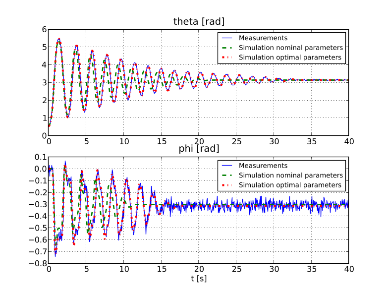
Steady-state Solver Interface for MATLAB® and Python🔗
Introduction🔗
The non-linear equation solver supports the solution of non-linear equation systems with discontinuities. The solver is based on the KINSOL solver that is a part of SUNDIALS. The primary application is the solution of steady-state model equations packaged into FMUs (Functional Mockup Units), see FMI2017. The solver utilizes interfaces provided by the FMI Toolbox for MATLAB®/Simulink (FMIT) and PyFMI (Python) respectively to interact with FMUs.
The solver is intended to be applied for non-linear equation systems on the form:
f(x,sw)=0
g(x,sw)...
Here x is a column vector of unknown length, sw are the current state of switches and f(x,sw) is a column vector of residuals. The number of residuals is equal to the number of unknowns. The equations are solved using an iterative equation solver starting with an initial guess for the iteration variables and accuracy is controlled both by the solver options and nominal values for the iteration variables.
The equations may contain discontinuities that are identified with discontinuity indicator functions g(x, sw), which are real-valued functions. Discontinuities occur when an indicator function changes sign. The residual functions are expected to be at least C1 continuous outside the discontinuities represented by the indicator functions. This implies that there are two separate continuous representations of f(x, sw) around each discontinuity. Explicit callback function is utilized by the solver to switch between the two continuous representations around a discontinuity.
Working with the Steady-State Solver MATLAB® and Python Interfaces🔗
Working with the steady-state interface involves setting up problems, e.g. by compiling Modelica models into FMUs, and feeding these to the solver. When the solver solves it actively reports information, which makes it easy to quickly monitor and understand what happens. Once the solver is finished it has created a log file with extensive information about the solution progress, much more detailed than what was provided during the solver process. This information can be used to understand in detail what happened, which is for example useful for debugging non-convergence and finding enhancements. To this end the steady-state solver in MATLAB® and Python ships with a logging functionality that interprets the generated log files and provides an information retrieval API.
To use the steady-state interface Problem and Solver instances must be created, where the Problem is given as an argument to the Solver constructor. A typical use case in MATLAB® will include an FMUProblem instance that is created by supplying an FMUModelME1 or CoupledFMUModelME1 model instance, as provided by FMIT and OCT, as an argument to the FMUProblem constructor. Corresponding in Python is to provide the FMUProblem constructor with an FMUModelME2 from PyFMI. FMUProblem is a subclass of the Problem class that is included in the package, and it uses FMUs that follow the input and output variable conventions as generated when using the Modelica compiler provided by OCT. It is also possible to create custom subclasses of the Problem class and provide them to the Solver. The log information retrieval API is provided through the LogViewer class.
Below a short description of the API is given, followed by some examples: a simple use case, a complete use case including specification of a Modelica model and compilation to an FMU using the Modelica compiler provided by OCT, an example showing how to use the information retrieval API, an example showing how to create a custom subclass to Problem and finally an example demonstrating the concept of interactive FMUs.
For Python, the examples below are equivalent to whether a 32-bit or 64-bit version is used. For MATLAB® users this holds only for a 64-bit version. Moreover, the bitness of the solvers is tied to the specific bitness of Python or MATLAB® that is used. Note that FMUs are platform-specific, and need to be compiled for the platform used.
Important Interface Features🔗
Described below are some central user aspects of the Problem, Solver and LogViewer classes. The mechanics of log file creation is also described. The classes are located inside the MATLAB® package oct.nlesol and Python package oct.steadystate.nlesol respectively.
For detailed documentation about classes and methods use interactive documentation. In MATLAB® this can be retrieved through:
• help CLASS_NAME For class level help.
• help CLASS_NAME.METHOD_NAME For detailed documentation about methods.
• doc CLASS_NAME Explore documentation using MATLAB® documentation browser.
In Python, this can be retrieved through:
• help(object) can be utilized to access docstrings. For example by typing in a Python-shell: help(Solver).
• object?, e.g. Solver?, can also be utilized to access docstrings if using IPython or PyLab.
Note that the solver uses Math Kernel Library (MKL) and that it can slightly affect the results of a solution. For further information, see Section C.5 in OPTIMICA Compiler Toolkit User's guide.
Problem and FMUProblem🔗
The Problem class in itself can not be used with the solver as it provides no way to populate it with problem information. The intended use is via subclasses, either through a custom implementation or by using the provided class FMUProblem, which uses interactive FMUs. An interactive FMU is designed to expose the system to an external solver, and this is achieved by transforming the iteration variables to inputs and the residual variables to outputs on the FMU, see the example in Interactive FMU below for further details.
FMUProblem takes an FMU as an argument to the constructor, and it may also take names of iteration and residual variables. FMUProblem provides functionality to hold iteration variables and residuals, see examples in the section called “Hold Iteration Variables (Python)” and the section called “Hold Iteration Variables (MATLAB)”. FMUProblem also provides functionality for parametric holding, see examples in the section called “Parametric Hold Iteration Variables (Python)” and the section called “Parametric Hold Iteration Variables (MATLAB)” and see Specification of Hand Guided Tearing for a specification of how parametric holding is specified in models.
FMUProblem supports handling of initial guess based on iteration variable start attribute that is symmetric to the handling done in FMUs with an integrated solver. Specifically, if the start attribute is defined via a parametric expression the expression is evaluated and used during FMU initialization. See the example in the section called “Parametric Start Attributes (MATLAB)” for more details.
A convenient way to view information about the FMUProblem is through the printInfo and print_info methods for MATLAB® and Python respectively.
Solver🔗
Solver takes a Problem instance as an argument to the constructor. This instance represents the steady-state problem to be solved. The most important methods are the solve method, which invokes the solver, and the setOptions method in MATLAB® and the corresponding functionality with solve_options() and the options argument to the solve method in Python. Possible options for the solver are given in the table below.
| Option | Default | Description |
|---|---|---|
| active_bounds_mode | 0 | 0 - project Newton step, 1 - use steepest descent in case of non-descent direction. (Corresponding compiler option: nle_active_bounds_mode) |
| check_jac_cond | true | Calculate Jacobian condition number and write it out to the log. (Corresponding compiler option: nle_solver_check_jac_cond) |
| Brent_ignore_error | false | Ignore Brent solve error for debugging purposes. (Corresponding compiler option: nle_brent_ignore_error) |
| discontinuities_tolerance (MATLAB only) | 1e-10 | Tolerance used to decide if discontinuity was crossed [eps(1), 0.1] (Corresponding compiler option: None). |
| enforce_bounds | true | Enforce bounds on iteration variables flag (true/false) (Corresponding compiler option: enforce_bounds) |
| iteration_variable_scaling | 2 | Iteration variable scaling mode:0 - no scaling, 1 - heuristic scaling, 2 - nominal based scaling. (Corresponding compiler option: iteration_variable_scaling) |
| jacobian_calculation_mode | 0 | Mode for how to calculate the Jacobian: 0 - one sided differences, 1 - central differences, 2 - central differences at bound, 3 - central differences at bound and 0, 4 - central differences in second Newton solve, 5- central differences at bound in second Newton solve, 6 - central differences at bound and 0 in second Newton solve, 7 - central differences when small residual, 8 - calculate Jacobian through MATLAB®, 9 - Jacobian compression. (Corresponding compiler option: nle_jacobian_calculation_mode) |
| jacobian_check | false | Compare the Jacobian calculated through MATLAB® with the finite differences Jacobian. (Corresponding compiler option: None) |
| jacobian_check_tolerance | 1e-6 | Maximal allowed relative error between the Jacobians compared through option 'check_jacobian' [eps(1), 1] (Corresponding compiler option: None) |
| jacobian_finite_difference_delta | sqrt(eps) | Delta to use when calculating finite difference Jacobians [eps(1), 0.1] (Corresponding compiler option: nle_jacobian_finite_difference_delta) |
| jacobian_update_mode | 2 | Mode for how to update the Jacobian: 0 - full Jacobian, 1 - Broyden update, 2 - reuse Jacobian (Corresponding compiler option: nle_jacobian_update_mode) |
| log_level | 4 | Log level for the solver [0, 8] (Corresponding compiler option: log_level) |
| max_iter | 100 | Maximum number of iterations in the non-linear solver [1, 1000] (Corresponding compiler option: nle_solver_max_iter) |
| max_iter_no_jacobian | 10 | Maximum number of iterations without Jacobian update. Value 1 means an update in every iteration. [1, 1000] (Corresponding compiler option: nle_solver_max_iter_no_jacobian) |
| max_residual_scaling_factor | 1e10 | Maximum allowed scaling factor for residuals [1, 1e32] (Corresponding compiler option: nle_solver_max_residual_scaling_factor) |
| min_residual_scaling_factor | 1e-10 | Minimal allowed scaling factor for residuals [1e-32, 1] (Corresponding compiler option: nle_solver_min_residual_scaling_factor) |
| regularization_tolerance | 1e-10 | Tolerance for deciding when Jacobian regularization should kick in (i.e. when condition number is larger than 1/regularization_tolerance [eps(1), 0.1] (Corresponding compiler option: nle_solver_regularization_tolerance) |
| rescale_after_singular_jac | true | Update scaling factors after passing a singular point. (Corresponding compiler option: rescale_after_singular_jac) |
| rescale_each_solve | false | Update scaling factors at the beginning of each solve() call. (Corresponding compiler option: rescale_each_step) |
| residual_equation_scaling | 1 | Residual equation scaling mode: 0 - no scaling, 1 - automatic scaling, 2 - manual scaling, 3 - hybrid scaling, 4 - aggressive automatic scaling, 5 - automatic rescaling at full Jacobian update. (Corresponding compiler option: residual_equation_scaling) |
| solver_exit_criterion | 3 | Exit criterion mode for the solver: Valid values: 0 - step length and residual based, 1 - only step length based, 2 - only residual based, 3 - hybrid. (Corresponding compiler option: nle_solver_exit_criterion) |
| tolerance | 1e-6 | Relative tolerance [eps(1), 0.1]. (Corresponding compiler option: nle_solver_default_tol) |
| silent_mode | false | No solve information written to the screen, but still to log (true/false) (Corresponding compiler option: None). |
| step_limit_factor | 0.2 | Factor used to limit the step size based on nominal and min/max range [0.01, 100]. Newton step length is limited so that for any iteration variable xi it is not larger than step_limit_factor times min(max(abs(nominal), abs(xi)),(xi_max-xi_min)). (Corresponding compiler option: nle_solver_step_limit_factor) |
| use_Brent_in_1d | false | Use Brent as a backup method for solving 1D equations. (Corresponding compiler option: use_Brent_in_1d) |
| use_jacobian_equilibration | false | Use Jacobian equilibration to improve linear solver accuracy (true/false). (Corresponding compiler option: use_jacobian_equilibration) |
As the solver progresses it will print out status messages to the MATLAB® terminal/Python console. These are provided to give a quick overview of the process.
LogViewer🔗
LogViewer works with log files, both from logs generated by the Solver and logs generated by FMIT and PyFMI, during e.g. initialization. In the case of logs generated by the Solver they are stored as XML files. Log files generated by FMIT and PyFMI are stored as .txt files that contain XML data. The log files contain a lot of information, and the amount of information saved in them can be regulated by setting the log level on the Solver and on the FMUs, see How to Control Information Saved in Log Files for further details. LogViewer provides an API for retrieving information from the log. Example of methods it provides are in the MATLAB® case: getIterationVariables, getResiduals, getJacobian, getErrors, getStep and getWarnings. Corresponding Python methods are: get_iteration_variables, get_residuals, get_jacobian, get_errors, get_step and get_warnings.
A LogViewer can be created either by providing a Solver object or the name of a log file as an argument to the constructor.
How to Control Information Saved in Log Files🔗
The OCT steady-state packages contain a powerful logging framework. The framework is particularly useful when applied to FMUs compiled with OCT Modelica compiler. This section will explain how to determine what data should be logged. It may be necessary to determine what data is logged for large models, since logging can use a lot of resources.
When using oct.nlesol with FMIT in MATLAB® there are three ways to change what log data will be saved:
• Set an option on the oct.nlesol.Solver object.
• Give an argument to the constructor of the FMIT FMU object.
• Set a parameter on the FMU.
When using oct.steadystate.nlesol in Python together with PyFMI there are three ways to change what log data will be saved:
• Provide an option on the oct.steadystate.nlesol.Solver object.
• Give the argument log_level to PyFMI's load_fmu.
• Set a parameter on the FMU.
These values will change different aspects of what is logged, and they may also affect each other. Below an overview of these ways and their connections is presented. Note that the logging framework can also be used with logs produced by FMUs with an integrated solver, in that case, the log level can only be changed directly on the FMU as no Solver object is used.
Events that trigger logging mostly include the solution of equations blocks, but also other information such as ModelicaMessage/ModelicaError in external C-libs, IO messages about external files such as XML files used by the FMU and asserts in Modelica code. There are two places where equation blocks may be solved:
• In the segregated MATLAB®/Python solver.
• In code that is built into the FMU.
In the case of FMUs with an integrated solver, blocks are only solved inside the FMU. For FMUs used together with the segregated MATLAB®/Python solver, blocks are typically solved only in the segregated solver. When solving FMUs with local iterations, the blocks for local iterations are solved inside the FMU even if the segregated solver is used. The blocks for local iterations are typically solved using a Brent solver.
In MATLAB® the log level can be set by:
• Solver.setOptions('log_level'): For the segregated solver this is the main log level and will determine what data is emitted about the block solved by the segregated solver. This will not affect what data is emitted by the FMU.
• As a parameter on the FMU: fmu.setValue(‘_log_level’, nnn), where nnn is an integer. The log level can only be changed before a call to fmiInitialize. Since fmiInitalize is called on the FMU as part of the FMUProblem constructor it can only be set before the FMUProblem is created. The default log level for an FMU is set with a compiler option ‘log_level’.
• In the constructor to an FMIT FMU object, e.g. fmu = FMUModelME1(fmuName, ‘log_level’) . Where log_level is: 'all', 'verbose', 'info', 'warning', 'error', 'fatal', 'nothing'. See FMIT docs for further details. In Python the log level can be set by:
• Changing the solver option log_level by first retrieving a SolverOptions object through
opts = solver.solve_options()
Then the log level is set through:
opts['log_level'] = val
and opts is passed to the solve(options=opts) method. It is also possible to set the log level without retrieving a SolverOptions object using solve(options = {'log_level': val}) where val is a suitable integer.
This affects what data is emitted about the block solved by the segregated solver and does not affect what data is emitted by the FMU.
• As a parameter on the FMU: fmu.set("_log_level", nnn), where nnn is an integer. The log level can only be changed before a call to initialize. Since initialize is called on the FMU as part of the FMUProblem constructor it can only be set before the FMUProblem is created. The default log level for an FMU is set with a compiler option ‘log_level’.
• Invoking the command load_fmu(fmu_name, log_level=XX) and setting XX to any integer in the range zero to seven.
With PyFMI it is also possible to set the log level of a model that has already been loaded, this is done by using the set_log_level(param) method. E.g. model.set_log_level(7).
As mentioned above, the log level set on the solver object does not affect the log information emitted by the FMU. However, in MATLAB® the log level set as an argument to the constructor of the FMIT FMU object affects what happens when the log level is set as a parameter on the FMU. The constructor log level determines what information can be logged by the FMU. For example, if it is set to ‘warning’ then only log messages that are considered warnings or more severe can be logged by the FMU. Thus setting a very high log level as a parameter on the FMU would not give a log with much information if FMIT log level is not set at the same time. Examples:
fmu = loadFMU(fmuName, ‘error’).
fmu.setValue('_log_level', 8) % No effect of high log level since only errors are passed
 through by FMIT
fmu.setValue('_log_level', 0) % No information emitted by the FMU

fmu = loadFMU(fmuName, 'all')
fmu.setValue('_log_level', 8) % All possible information emitted by the FMU
fmu.setValue('_log_level', 0) % No information emitted by the FMU
In PyFMI, the log_level that is set either as an argument to the load_fmu method or through fmu.set_log_level() determines what information will be passed through. That means, like in the MATLAB® case above that:
fmu = load_fmu(fmu_name, log_level=2)
fmu.set('_log_level', 8) # No effect of high log level since only errors are passed through
 by PyFMI
fmu.set('_log_level', 0) # No information emitted by the FMU

fmu = load_fmu(fmuName, log_level=7)
fmu.set('_log_level', 8) % All possible information emitted by the FMU
fmu.set('_log_level', 0) % No information emitted by the FMU
To get information about the blocks solved in the FMU the log level set in the constructor must be ‘info’/4 or above. Messages that are considered ‘info’/4 include all types of information emitted in the solution of blocks. So if an FMU object is created with log level ‘info’/4 then the log level set as a parameter on the FMU determines exactly what messages on the level of info that are emitted. For example, to get full information from the blocks solved by Brent requires log level 8. But if blocks are solved using a Newton solver only log level 6 is needed.
What Log Files are Created🔗
There are two different log files written for a ModelA.fmu compiled from ModelA in Modelica:
• ModelA_log.txt – produced by FMIT/PyFMI. The detail level is controlled by setting the log level on the FMU in one of the two ways described above. The log can be used by LogViewer which retrieves and parses the XML information in the file. This is used when the system is solved with an integrated solver.
• ModelA_log.xml (MATLAB)/ModelA_solver_log.xml (Python) – produced by LogMonitor in MATLAB®/Python segregated solver. Detail level is controlled by log_level option of the solver, and by the log level set on the FMU as detailed above. The log can be used by LogViewer, which parses the XML information in the file.
Control Log Information with Log Level🔗
A summary of the OCT log levels and what information they are associated with is given below:
• 0: Log nothing
• 1: Errors
• 2: Warnings
• 3: Base-line information
• 4: Detailed information including basic Newton solver traces
• 5: Detailed information including Newton solver traces
• 6: Detailed information including Jacobians
• 7: Detailed information including basic information on Brent
• 8: Detailed information including Brent traces
Examples🔗
In this section we show examples similar for both Python and MATLAB®, starting with Python and continuing with MATLAB®. These examples cover basic functionality such as solving the problem, creating custom problems, working with the LogViewer, and parametric holding. The aim of this section is to familiarize the user with the procedure of using FMUs for steady-state solving and accessing the results by means of basic examples.
First we will, however, go through some concepts which are shared between Python and MATLAB®; how to create an interactive FMU and how to interpret the solver trace.
Interactive FMU🔗
This example shows how the compiler creates an FMU from a steady-state Modelica model. The model:
model twoEqSteadyState
    Real x (start = 1);
    Real T (start = 400);
equation
    0 = 120*x - 75*(0.12*exp(12581*(T - 298)/(298*T)))*(1 - x);
    0 = -x*(873 - T) + 11.0*(T - 300);
end twoEqSteadyState;
Compiling this model with the interactive fmu option set to true will produce the following flattened model:
fclass twoEqSteadyState
    input Real x(start = 1);
    input Real T(start = 400);
    parameter Real iter_0 "T";
    output Real res_0(nominal = 0) "0 = (- x) * (873 - T) + 11.0 * (T - 300)";
    parameter Real iter_1 "x";
    output Real res_1(nominal = 0) "0 = 120 * x - 75 * (0.12 * exp(12581 * (T - 298) / (298 *
    T))) * (1 - x)";
parameter equation
    iter_0 = 400;
    iter_1 = 1;
equation
    res_1 = 75 * (0.12 * exp(12581 * (T - 298) / (298 * T))) * (1 - x) - 120 * x;
    res_0 = - (- x) * (873 - T) - 11.0 * (T - 300);
end twoEqSteadyState;
Where we see that the iteration variables are now inputs and there are residual variables as outputs.
Interpreting the Solver Trace🔗
A typical solver trace generated (in this case from the MATLAB® example in the section called “Complete Example (MATLAB)”) by the steady-state solver looks like:
Model name.........................: ExampleModels.SimpleSteadyState
Number of iteration variables......: 1
Number of discontinuity switches...: 2

Switch iteration 1
iter        res_norm       max_res: ind   nlb  nab   lambda_max: ind      lambda
   1Js    1.0000e+00   1.0000e+00:   1     0    0   2.0000e-01:   1r  2.0000e-01
   2      8.0000e-01   8.0000e-01:   1     0    0   2.0000e-01:   1r  2.0000e-01
   3      6.4000e-01   6.4000e-01:   1     0    0   2.0000e-01:   1r  2.0000e-01
   4      5.1200e-01   5.1200e-01:   1     0    0   2.0000e-01:   1r  2.0000e-01
   5      4.0960e-01   4.0960e-01:   1     0    0   2.4414e-01:   1r  2.4414e-01
   6      3.0960e-01   3.0960e-01:   1     0    0   3.2300e-01:   1r  3.2300e-01
   7      2.0960e-01   2.0960e-01:   1     0    0   4.7710e-01:   1r  4.7710e-01
   8      1.0960e-01   1.0960e-01:   1     0    0   9.1241e-01:   1r  9.1241e-01
   9      9.6000e-03   9.6000e-03:   1     0    0   1.0000e+00        1.0000e+00
   10     0.0000e+00   0.0000e+00:   1
iter        res_norm       max_res: ind   nlb  nab   lambda_max: ind      lambda
   1s     0.0000e+00   0.0000e+00:   1
Switch iteration 2
iter        res_norm      max_res:  ind   nlb  nab   lambda_max: ind      lambda
   1      6.6667e-01   6.6667e-01:   1     0    0   3.0000e-01:   1r  3.0000e-01
   2      6.0000e-01   6.0000e-01:   1     0    0   3.3333e-01:   1r  3.3333e-01
   3      5.3333e-01   5.3333e-01:   1     0    0   3.7500e-01:   1r  3.7500e-01
   4      4.6667e-01   4.6667e-01:   1     0    0   4.2857e-01:   1r  4.2857e-01
   5      4.0000e-01   4.0000e-01:   1     0    0   5.0000e-01:   1r  5.0000e-01
   6      3.3333e-01   3.3333e-01:   1     0    0   6.0000e-01:   1r  6.0000e-01
   7      2.6667e-01   2.6667e-01:   1     0    0   9.0000e-01:   1r  9.0000e-01
   8      1.8667e-01   1.8667e-01:   1     0    0   1.0000e+00        1.0000e+00
   9      1.2444e-01   1.2444e-01:   1     0    0   1.0000e+00        1.0000e+00
   10J    8.2963e-02   8.2963e-02:   1     0    0   1.0000e+00        1.0000e+00
   11J    2.8553e-10  -2.8553e-10:   1     0    0   1.0000e+00        1.0000e+00
   12     0.0000e+00   0.0000e+00:   1
Switch iteration 3
iter        res_norm      max_res:  ind   nlb  nab   lambda_max: ind       lambda
 1        6.6667e-01  -6.6667e-01:   1     0    0   2.0000e-01:   1r   2.0000e-01
 2        2.6667e-01  -2.6667e-01:   1     0    0   4.0000e-01:   1r   4.0000e-01
 3        5.3333e-02   5.3333e-02:   1     0    0   1.0000e+00         6.0000e-01
 4        4.2667e-02  -4.2667e-02:   1     0    0   1.0000e+00         6.0000e-01
 5        3.4133e-02   3.4133e-02:   1     0    0   1.0000e+00         6.0000e-01
 6        2.7307e-02  -2.7307e-02:   1     0    0   1.0000e+00         6.0000e-01
 7        2.1845e-02   2.1845e-02:   1     0    0   1.0000e+00         6.0000e-01
 8        1.7476e-02  -1.7476e-02:   1     0    0   1.0000e+00         6.0000e-01
 9        1.3981e-02   1.3981e-02:   1     0    0   1.0000e+00         6.0000e-01
 10J      1.1185e-02  -1.1185e-02:   1     0    0   1.0000e+00         1.0000e+00
 11J      7.5318e-11   7.5318e-11:   1     0    0   1.0000e+00         1.0000e+00
 12       7.4015e-17   7.4015e-17:   1
Number of function evaluations: 60
Number of jacobian evaluations: 5
Solver finished
Total time in solver: 0.35 s
The solver outputs brief progress messages to allow to follow the solution progress in real-time. Solution is performed using a sequence of Newton iterations; each produces a line of status values. Newton iterations are grouped into runs that start from iteration number iter=1 (which gives status before the first iteration). Each run of Newton iterations belongs to a switch iteration, printed as a header.
iter gives the number of the current Newton iteration in the current run. It can be followed by one or more letters:
• J: The Jacobian was updated at the beginning of the iteration.
• s: The residual scaling was updated at the beginning of the iteration.
• r: Regularization is used during the iteration due to a singular Jacobian.
• x: Iteration was retried due to line search failure and Jacobian not up-to-date.
• m: A minimum norm approach was used to calculate the step.
• d: Steepest descent direction used.
res_norm is the 2-norm of the current residual according to the current residual scaling. max_res is the value of the scaled residual that currently has the greatest magnitude, and the corresponding ind is its index.
At the start of each Newton iteration, the solver computes a Newton step based on the current residuals and Jacobian. The search direction is updated to move along active variable bounds and the step length is limited based on the two criteria:
• Limiting bounds: full step violates min/max bounds on some iteration variables.
• Range limit: full step length in a variable is too long as compared to the variable specific range limit based on nominal value and max-min range (see step_limit_factor solver option).
nlb column gives the current number of limiting bounds including active ones, and nab gives the number of active bounds. Line search is performed with the (projected) Newton step as search direction; the actual step taken is lambda times the (projected) Newton step.
The lambda_max value gives the upper bound on lambda from the step limiting criteria. The index of the most limiting variable in the block is given by the corresponding ind, if there is one. The r suffix indicates that the range limit condition reduced the step the most. The step length may be further reduced as a part of line-search if lambda_max does not give sufficient residual decrease.
The step lengths and number of limiting/active bounds reported on an iteration are for the step that is taken at the iteration. This is why they are not printed at the last iteration.
Python Examples🔗
Introductory Example (Python)
The simple introductory example below shows how an FMUProblem instance is created, where PyFMI is used to load an FMU model. A solver instance is created from the FMUProblem instance, and the steady-state solver is invoked.
 from pyfmi import load_fmu
 from oct.steadystate.nlesol import FMUProblem, Solver
 fmu_model = load_fmu('SteadyStateProblem.fmu')
 fmu_problem = FMUProblem(fmu_model)
 solver = Solver(fmu_problem)
 sol = solver.solve()
Complete Example (Python)
This model is included in ExampleModels.mo-package, and to run this example begin by importing the example by
from oct.steadystate.examples import simple_steadystate
and then run
simple_steadystate.run_demo()
First, create a steady-state Modelica model and save it to a file SimpleSteadyState.mo.
model SimpleSteadyState
 parameter Real a = 2;
 input Real b(start = 2);
 Real x (start = -2);
equation
 b = if (x < -1.0)
   then x + (x + 1)*a
  else
   if (x > 1)
    then x + (x - 1)*a
   else
    x;
end SimpleSteadyState;
Next we compile the FMU with the required interactive argument and imports.
import os
import numpy as np
from pymodelica import compile_fmu
from pyfmi import load_fmu
from oct.steadystate.nlesol import FMUProblem, Solver
compiler_opts = {"interactive_fmu": True,
     "expose_scalar_equation_blocks_in_interactive_fmu": True}
name = compile_fmu("SimpleSteadyState",
     "SimpleSteadyState.mo",
     compiler_options=compiler_opts)
Next we use PyFMI to load the FMU and pass the FMUModelME2 instance to FMUProblem.
model = load_fmu(name, log_level=4)
problem = FMUProblem(model)
Note that it is also possible to supply the names of iteration and residual variables when the FMUProblem is created, for the model above the following would have worked as well:
problem = FMUProblem(model, iteration_variables=["x"], residual_variables=["res_0"])
This feature is useful when not all iteration and residual variables in an interactive FMU are used. Next, we create a Solver instance and invoke the steady-state solver.
solver = Solver(problem)
res = solver.solve()
When calling for the solve() command, it produces the following output (described in more detail in Interpreting the Solver Trace).
Model name..............................: ExampleModels.SimpleSteadyState
Number of iteration variables...........: 1
Number of discontinuity switches........: 2

Event iteration 1
iter       res_norm       max_res: ind   nlb  nab   lambda_max: ind      lambda
   0Js   1.0000e+000  1.0000e+000:  0     0    0   2.0000e-001:  0r 2.0000e-001
   1     8.0000e-001  8.0000e-001:  0     0    0   2.0000e-001:  0r 2.0000e-001
   2     6.4000e-001  6.4000e-001:  0     0    0   2.0000e-001:  0r 2.0000e-001
   3     5.1200e-001  5.1200e-001:  0     0    0   2.0000e-001:  0r 2.0000e-001
   4     4.0960e-001  4.0960e-001:  0     0    0   2.4414e-001:  0r 2.4414e-001
   5     3.0960e-001  3.0960e-001:  0     0    0   3.2300e-001:  0r 3.2300e-001
   6     2.0960e-001  2.0960e-001:  0     0    0   4.7710e-001:  0r 4.7710e-001
   7     1.0960e-001  1.0960e-001:  0     0    0   9.1241e-001:  0r 9.1241e-001
   8     9.6000e-003  9.6000e-003:  0     0    0   1.0000e+000      1.0000e+000
   9     0.0000e+000  0.0000e+000:  0
iter       res_norm       max_res: ind   nlb  nab   lambda_max: ind      lambda
   0s    0.0000e+000  0.0000e+000:  0
Event iteration 2
iter       res_norm       max_res: ind   nlb  nab   lambda_max: ind      lambda
   0     6.6667e-001  6.6667e-001:  0     0    0   3.0000e-001:  0r 3.0000e-001
   1     6.0000e-001  6.0000e-001:  0     0    0   3.3333e-001:  0r 3.3333e-001
   2     5.3333e-001  5.3333e-001:  0     0    0   3.7500e-001:  0r 3.7500e-001
   3     4.6667e-001  4.6667e-001:  0     0    0   4.2857e-001:  0r 4.2857e-001
   4     4.0000e-001  4.0000e-001:  0     0    0   5.0000e-001:  0r 5.0000e-001
   5     3.3333e-001  3.3333e-001:  0     0    0   6.0000e-001:  0r 6.0000e-001
   6     2.6667e-001  2.6667e-001:  0     0    0   9.0000e-001:  0r 9.0000e-001
   7     1.8667e-001  1.8667e-001:  0     0    0   1.0000e+000      1.0000e+000
   8     1.2444e-001  1.2444e-001:  0     0    0   1.0000e+000      1.0000e+000
   9J    8.2963e-002  8.2963e-002:  0     0    0   1.0000e+000      1.0000e+000
   10    2.8553e-010 -2.8553e-010:  0     0    0   1.0000e+000      1.0000e+000
   11    0.0000e+000  0.0000e+000:  0
Event iteration 3
iter       res_norm       max_res: ind   nlb  nab   lambda_max: ind      lambda
   0     6.6667e-001 -6.6667e-001:  0     0    0   2.0000e-001:  0r 2.0000e-001
   1     2.6667e-001 -2.6667e-001:  0     0    0   4.0000e-001:  0r 4.0000e-001
   2     5.3333e-002  5.3333e-002:  0     0    0   1.0000e+000      6.0000e-001
   3     4.2667e-002 -4.2667e-002:  0     0    0   1.0000e+000      6.0000e-001
   4     3.4133e-002  3.4133e-002:  0     0    0   1.0000e+000      6.0000e-001
   5     2.7307e-002 -2.7307e-002:  0     0    0   1.0000e+000      6.0000e-001
   6     2.1845e-002  2.1845e-002:  0     0    0   1.0000e+000      6.0000e-001
   7     1.7476e-002 -1.7476e-002:  0     0    0   1.0000e+000      6.0000e-001
   8     1.3981e-002  1.3981e-002:  0     0    0   1.0000e+000      6.0000e-001
   9J    1.1185e-002 -1.1185e-002:  0     0    0   1.0000e+000      1.0000e+000
   10    7.7968e-011  7.7968e-011:  0     0    0   1.0000e+000      1.0000e+000
   11    7.4015e-017  7.4015e-017:  0
Number of function evaluations..........: 56
Number of jacobian evaluations..........: 3
Solver finished
Total time in solver....................: 0.22 s
Note that indexing of iteration variables and residuals starts from 0 here in Python instead of 1 as compared to MATLAB®.
Log Information Retrieval (Python)
Below an example is presented where a steady-state problem is solved and the generated log-file provided to the LogViewer. This model is included in the ExampleModels.mo-package and the corresponding script to run it is in log_viewer.py.
compiler_opts = {"interactive_fmu": True,
                 "expose_scalar_equation_blocks_in_interactive_fmu": True}
name = compile_fmu("ExampleModels.twoEqSteadyState",
                   os.path.join(curr_dir, "files", "example_models.mo"),
                   compiler_options=compiler_opts)

# Use pyfmi to create an fmu model object.
model = load_fmu(name, log_level=4)
model.set("_log_level", 4)

# Create the problem class instance from the fmu and supply it to the
# solver.
problem = FMUProblem(model)
solver = Solver(problem)

# Solve the problem with a log level sufficiently high to get
# values of iteration variables emitted to the log file.
solver.solve({"log_level": 6})

# Create the LogViewer from the solver class instance we
# created above as such
log_viewer = LogViewer(solver)

# LogViewer can also be supplied with the log-file, e.g.
# log_viewer = LogViewer("twoEqSteadyState_log.xml")

# It is now possible to play around and retrieve information from the log.
# E.g. retrieve the values of the iteration variables at different
# times during the solver invocation.
iter_data_second_newton = log_viewer.get_iteration_variables()
iv_names = log_viewer.get_iteration_variable_names()[0]
residuals = log_viewer.get_residuals()

if with_plots:
    import matplotlib.pyplot as plt
    # Plot the data
    f, (ax1, ax2, ax3) = plt.subplots(3, sharex=True)
    ax1.plot(iter_data_second_newton[0][:, :])
    ax1.margins(0,0.1)
    ax1.set_title("IV values as a function of iterations in Newton solve invocation")
    ax1.set_ylabel("Values")
    ax1.legend(iv_names)
    ax2.semilogy(np.abs(iter_data_second_newton[0][:, :]-iter_data_second_newton[0][-1, :]))
    ax2.margins(0,0.1)
    ax2.set_ylabel("Distance")
    ax3.semilogy(np.abs(residuals[0]))
    ax3.set_ylabel("Residuals")
    ax3.set_xlabel("Iteration #")
    plt.tight_layout()

# For several functions one may specify which iteration variables one is interested in.
nominal_data_second_newton =
 log_viewer.get_iteration_variable_nominal(iv_names=[iv_names[0]])

# Retrieve the solver trace
solver_trace = log_viewer.get_solver_trace()


# If the steady-state solver was used several times on the same problem it will have
# filled the log file with information from the different solver invocations. To get
# information about a particular solver invocation and/or solve provide the solve index
# as argument. Solve indices can be found through
print("Solve info:")
print(log_viewer.get_solve_info())

# E.g. to get the values of iteration variables for the second
# solver invocation log present in the log the following is used:
# Solve index is 2 since two Newton solves have been performed in solver invocation 0.
iter_data_second_newton = log_viewer.get_iteration_variables(2)
# Or to only get information for a particular variable
iter_data_second_newton = log_viewer.get_iteration_variables(2, iv_names=[iv_names[0]])

# Other functions provided by LogViewer
res_var_data_second_newton = log_viewer.get_residuals()
res_data_second_newton = log_viewer.get_scaled_residual_norm()
jac_data_second_newton = log_viewer.get_jacobians()
iter_num_second_newton = log_viewer.get_number_of_iterations()

# For some of LogViewer's functions it is possible to specify a solve index
# together with an iteration number to retrieve data only from there.
# Note from the get_solve_info() output that solve index represents a Newton
# solve
newton_step = log_viewer.get_step("Newton", 1, 0, scaled_step=False)
lambda_max = log_viewer.get_step_ratio("lambda_max", 1, 0)
The following plot was generated in the example:
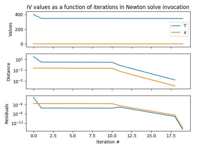
Creating Custom Problem Class (Python)
It is also possible to implement custom subclasses by utilizing inheritance of the Problem class. Below we show a complete class.
# Solving:
# FX = if(x < -1)
#         x + (x+1)*COEFF;
#      else
#          if(x > 1)
#              x + (x - 1)*COEFF;
#          else
#              x;

import numpy as np
from oct.steadystate.nlesol.problem import Problem

class TestProblem(Problem):


 def __init__(self):
  Problem.__init__(self)
  self.FX = 2
  self._COEFF = 2
  self._n_iteration_variables = 1
  self._n_discontinuity_indicators = 2
  self._x_initial = np.array([2])
  self._x = self._x_initial
  self.sw0 = False
  self.sw1 = False


def get_number_of_iteration_variables(self):
 return self._n_iteration_variables

def get_number_of_discontinuity_indicators(self):
 return self._n_discontinuity_indicators

def get_initial_guess(self):
 return np.array([self._x_initial])

def get_iteration_variables(self):
 return np.array([self._x_initial])

def evaluate_discontinuity_indicators(self, ivs = None):
 if ivs is None:
  ivs = self._x
 return np.array([-ivs[0] - 1, ivs[0] - 1])

def make_discontinuous_change(self):
 self.sw0 = np.all(np.less(self._x, -1))
 self.sw1 = np.all(np.greater(self._x, 1))

def set_iteration_variables(self, x):
 self._x = x

def evaluate_residuals(self, x):
 if self.sw0:
  val = x + (x + 1)*self._COEFF
 elif self.sw1:
  val = x + (x - 1)*self._COEFF
 else:
  val = x
 return_val = self.FX - val
  self.set_iteration_variables(x)
 return return_val
This class can then be sent to the solver in much the same manner as above:
from oct.steadystate.nlesol import Solver
problem = TestProblem()
solver = Solver(cls.problem)
Hold Iteration Variables (Python)
In this example, we show the functionality of holding iteration variables for FMUProblem. It uses the model from Interactive FMU, which is included in the ExampleModels.mo-package. The Python script to run this example is hold_IVs.py. Interactive FMU
 # The FMUProblem in this example contains two iteration variables. Using
 # printInfo its structure is shown:

 problem.print_info()
 :::::::: Iteration variables ::::::::
    1: 4.0000000000000000E+02 T
    2: 1.0000000000000000E+00 x
 :::::::: Residual equations ::::::::
    0: -6.2700000000000000E+02 0 = (- x) * (873 - T) + 11.0 * (T - 300)
    1: -1.2000000000000000E+02 0 = 120 * x - 75 * (0.12 * exp(12581 * (T - 298) / (298
 * T))) * (1 - x)

 # To hold an iteration variable the method "hold_iteration_variables" is
 # provided. Let's hold variable T
 problem.hold_iteration_variables([0])
 print('problem.hold_iteration_variables([0])')
 # We could also use {'T'} as an argument

 # Using printInfo again we see that T, and the corresponding residual
 # equation is removed.
 problem.print_info()

 problem.hold_iteration_variables([0])
 :::::::: Iteration variables ::::::::
    1: 1.0000000000000000E+00 x
 :::::::: Residual equations ::::::::
    1: -1.2000000000000000E+02 0 = 120 * x - 75 * (0.12 * exp(12581 * (T - 298) / (298
 * T))) * (1 - x)

 # To restore the system we can use the method "releaseIterationVariables"
 problem.release_iteration_variables([0])
 print('\nproblem.release_iteration_variables([0])')
 problem.print_info()

 problem.release_iteration_variables([0])
 :::::::: Iteration variables ::::::::
    0: 4.0000000000000000E+02 T
    1: 1.0000000000000000E+00 x
 :::::::: Residual equations ::::::::
    0: -6.2700000000000000E+02 0 = (- x) * (873 - T) + 11.0 * (T - 300)
    1: -1.2000000000000000E+02 0 = 120 * x - 75 * (0.12 * exp(12581 * (T - 298) / (298
 * T))) * (1 - x)

 # We can specify which residual eqautions that should be removed
 problem.hold_iteration_variables([1], [0]) # Remove T, and res. eq 1
 print('\nproblem.hold_iteration_variables([1], [0])')
 problem.print_info()

 problem.hold_iteration_variables([1], [0])
 :::::::: Iteration variables ::::::::
    0: 4.0000000000000000E+02 T
 :::::::: Residual equations ::::::::
    1: -1.2000000000000000E+02 0 = 120 * x - 75 * (0.12 * exp(12581 * (T - 298) / (298
 * T))) * (1 - x)

 # Most methods on FMUProblem also lets you specify if you want to apply the
 # method for active, held or all variables. Default is active.
 print('\nproblem.printInfo("held")')
 problem.print_info('held')

 problem.printInfo("held")
 :::::::: Iteration variables ::::::::
    1: 1.0000000000000000E+00 x
 :::::::: Residual equations ::::::::
    0: -6.2700000000000000E+02 0 = (- x) * (873 - T) + 11.0 * (T - 300)

 print('\nproblem.printInfo("all")')
 problem.print_info('all')

 problem.printInfo("all")
 :::::::: Iteration variables ::::::::
    0: 4.0000000000000000E+02 T
    1: 1.0000000000000000E+00 x
 :::::::: Residual equations ::::::::
    0: -6.2700000000000000E+02 0 = (- x) * (873 - T) + 11.0 * (T - 300)
    1: -1.2000000000000000E+02 0 = 120 * x - 75 * (0.12 * exp(12581 * (T - 298) / (298
 * T))) * (1 - x)

 # It also possible change min/max/nominal attributes on the iteration
 # variables. This can e.g. be used if the initial guess is close
 # to the solution, where tighter bounds provides additional
 # guidance to the solver. This may be particularly useful in case of
 # multiple solutions.
Parametric Hold Iteration Variables (Python)
In addition to manually held variables, there is functionality for setting up hold specifications based on parameters on the FMU. The Modelica compiler provided by OCT supports special annotations for marking variables for parametric holding, see Specification of Hand Guided Tearing for a complete specification. The basic methodology behind parametric holding is that iteration variables and residuals are bound to boolean parameters. When the problem is constructed, the variables and residuals bound to boolean parameters that are true are automatically held. Specification of Hand Guided Tearing
The model for this example is included in the ExampleModels.mo-package and the script to run the example is parametric_hold_IV.py. In the model, parameters for parametric holding is specified for the iteration variables and residuals as follows:
model twoEqSteadyStateParaHold
 Real x (start = 1);
 Real T (start = 400);
 parameter Boolean testHold1 = false;
 parameter Boolean testHold2 = false;
equation
 0 = 120*x - 75*(0.12*exp(12581*(T - 298)/(298*T)))*(1 - x)
  annotation(__Modelon(ResidualEquation(hold = testHold1,
   iterationVariable(hold = testHold2)=x), name = LongEq));
 0 = -x*(873 - T) + 11.0*(T - 300)
  annotation(__Modelon(ResidualEquation(hold = testHold2,
   iterationVariable(hold = testHold1)=T), name = LongEq2));
end twoEqSteadyStateParaHold;
We begin by setting up the problem.
import os
from pymodelica import compile_fmu
from pyfmi import load_fmu
from oct.steadystate.nlesol import FMUProblem

compiler_opts = {"interactive_fmu": True,
                 "expose_scalar_equation_blocks_in_interactive_fmu": True,
                 "hand_guided_tearing": True}
model_name = 'ExampleModels.twoEqSteadyStateParaHold'
name = compile_fmu(model_name, "/../files/example_models.mo",
compiler_options=compiler_opts)
model = load_fmu(name, log_level=4)
model.set("testHold1", True)

problem = FMUProblem(model)
Now utilizing print_info() we get the following.
 print('problem.print_info()')
 problem.print_info()

 problem.print_info()
 :::::::: Iteration variables ::::::::
    1: 1.0000000000000000E+00 x
 :::::::: Residual equations ::::::::
    0: -6.2700000000000000E+02 LongEq2

 print('problem.print_info("parametric_hold")')
 problem.print_info("parametric_hold")

 problem.print_info("parametric_hold")
 :::::::: Iteration variables ::::::::
    0: 4.0000000000000000E+02 T
 :::::::: Residual equations ::::::::
    1: -1.2000000000000000E+02 LongEq

 print('problem.print_info("all")')
 problem.print_info("all")

 problem.print_info("all")
 :::::::: Iteration variables ::::::::
    0: 4.0000000000000000E+02 T
    1: 1.0000000000000000E+00 x
 :::::::: Residual equations ::::::::
    0: -6.2700000000000000E+02 LongEq2
    1: -1.2000000000000000E+02 LongEq
MATLAB Examples
These examples assume that the +oct folder, as provided in the installation, is on the MATLAB® path. Some of the examples described are included in the install/MATLAB/examples/nlesol folder.
Introductory Example (MATLAB)
The simple introductory example below shows how an FMUProblem instance is created, where FMIT is used to load an FMU model. A solver instance is created from the FMUProblem instance, and the steady-state solver is invoked.
import oct.nlesol.*; % Import nlesol package.
fmu = FMUModelME1('SteadyStateProblem.fmu');
fmuProblem = FMUProblem(fmu);
solver = Solver(fmuProblem);
sol = solver.solve();
Complete Example (MATLAB)
This model is included in the ExampleModels.mo-package and the corresponding script to run it is example_SimpleSteadyState.m. In the first step, create a steady-state Modelica model and save it to a file SimpleSteadyState.mo.
model SimpleSteadyState
        parameter Real a = 2;
        input Real b(start = 2);
        Real x (start = -2);
    equation
        b = if (x < -1.0)
                then x + (x + 1)*a
            else
                if (x > 1)
                    then x + (x - 1)*a
                else
                    x;
end SimpleSteadyState;
Next, we compile the FMU with the required interactive argument using the MATLAB® OCT compiler interface.
import oct.modelica.*; % Import compiler package.
import oct.nlesol.*; % Import nlesol package.
modelName = 'ExampleModels.SimpleSteadyState';
compiler = 'OCT_Modelica'; % To compile with the OCT provided Modelica compiler that
                       % supports special handling of iteration and residual variables.
exampledir = fileparts(mfilename('fullpath')); % Path to example directory
lib = {[exampledir, '\ExampleModels.mo']}; % Absolute path to model

% The options needed for special handling of iteration and residual variables.
opt = {'interactive_fmu', true, 'expose_scalar_equation_blocks_in_interactive_fmu', true};
fmuName = compileFMU(modelName, compiler, 'libs', lib, 'options', opt);
Next, we use FMIT to create an FMU model instance. Note that we create an FMU for Model Exchange in order to match the FMU generated by the compiler.
fmu = FMUModelME1(fmuName);
fmuProblem = FMUProblem(fmu);
Note that it is also possible to supply the names of iteration and residual variables when the FMUProblem is created, for the model above the following would have worked as well:
fmuProblem = FMUProblem(fmu, {'x'}, {'res_0'});
This feature is useful when not all iteration and residual variables in an interactive FMU are used.
Next, we create a Solver instance and invoke the steady-state solver.
solver = Solver(fmuProblem);
solver.solve()
This will produce the following output (described in more detail in Interpreting the Solver Trace ).
Model name.........................: ExampleModels.SimpleSteadyState
Number of iteration variables......: 1
Number of discontinuity switches...: 2

Switch iteration 1
iter       res_norm       max_res: ind   nlb  nab   lambda_max: ind      lambda
   1Js   1.0000e+00   1.0000e+00:   1     0    0   2.0000e-01:   1r  2.0000e-01
   2     8.0000e-01   8.0000e-01:   1     0    0   2.0000e-01:   1r  2.0000e-01
   3     6.4000e-01   6.4000e-01:   1     0    0   2.0000e-01:   1r  2.0000e-01
   4     5.1200e-01   5.1200e-01:   1     0    0   2.0000e-01:   1r  2.0000e-01
   5     4.0960e-01   4.0960e-01:   1     0    0   2.4414e-01:   1r  2.4414e-01
   6     3.0960e-01   3.0960e-01:   1     0    0   3.2300e-01:   1r  3.2300e-01
   7     2.0960e-01   2.0960e-01:   1     0    0   4.7710e-01:   1r  4.7710e-01
   8     1.0960e-01   1.0960e-01:   1     0    0   9.1241e-01:   1r  9.1241e-01
   9     9.6000e-03   9.6000e-03:   1     0    0   1.0000e+00        1.0000e+00
   10    0.0000e+00   0.0000e+00:   1
iter       res_norm       max_res: ind   nlb  nab   lambda_max: ind      lambda
 ´ 1s    0.0000e+00   0.0000e+00:   1
Switch iteration 2
iter       res_norm       max_res: ind   nlb  nab   lambda_max: ind      lambda
   1     6.6667e-01   6.6667e-01:   1     0    0   3.0000e-01:   1r  3.0000e-01
   2     6.0000e-01   6.0000e-01:   1     0    0   3.3333e-01:   1r  3.3333e-01
   3     5.3333e-01   5.3333e-01:   1     0    0   3.7500e-01:   1r  3.7500e-01
   4     4.6667e-01   4.6667e-01:   1     0    0   4.2857e-01:   1r  4.2857e-01
   5     4.0000e-01   4.0000e-01:   1     0    0   5.0000e-01:   1r  5.0000e-01
   6     3.3333e-01   3.3333e-01:   1     0    0   6.0000e-01:   1r  6.0000e-01
   7     2.6667e-01   2.6667e-01:   1     0    0   9.0000e-01:   1r  9.0000e-01
   8     1.8667e-01   1.8667e-01:   1     0    0   1.0000e+00        1.0000e+00
   9     1.2444e-01   1.2444e-01:   1     0    0   1.0000e+00        1.0000e+00
   10J   8.2963e-02   8.2963e-02:   1     0    0   1.0000e+00        1.0000e+00
   11J   2.8553e-10  -2.8553e-10:   1     0    0   1.0000e+00        1.0000e+00
   12    0.0000e+00   0.0000e+00:   1
Switch iteration 3
iter       res_norm       max_res: ind   nlb  nab   lambda_max: ind      lambda
   1     6.6667e-01  -6.6667e-01:   1     0    0   2.0000e-01:   1r  2.0000e-01
   2     2.6667e-01  -2.6667e-01:   1     0    0   4.0000e-01:   1r  4.0000e-01
   3     5.3333e-02   5.3333e-02:   1     0    0   1.0000e+00        6.0000e-01
   4     4.2667e-02  -4.2667e-02:   1     0    0   1.0000e+00        6.0000e-01
   5     3.4133e-02   3.4133e-02:   1     0    0   1.0000e+00        6.0000e-01
   6     2.7307e-02  -2.7307e-02:   1     0    0   1.0000e+00        6.0000e-01
   7     2.1845e-02   2.1845e-02:   1     0    0   1.0000e+00        6.0000e-01
   8     1.7476e-02  -1.7476e-02:   1     0    0   1.0000e+00        6.0000e-01
   9     1.3981e-02   1.3981e-02:   1     0    0   1.0000e+00        6.0000e-01
   10J   1.1185e-02  -1.1185e-02:   1     0    0   1.0000e+00        1.0000e+00
   11J   7.5318e-11   7.5318e-11:   1     0    0   1.0000e+00        1.0000e+00
   12    7.4015e-17   7.4015e-17:   1
Number of function evaluations: 60
Number of jacobian evaluations: 5
Solver finished
Total time in solver: 0.35 s

solution = 1.3333
Log Information Retrieval (MATLAB)
Below an example is presented where a steady-state problem is solved and the generated log-file provided to the LogViewer. This model is included in the ExampleModels.mo-package and the corresponding script to run it is example_LogViewer.m. Here we assume that the model ExampleModels.twoEqSteadyState has been compiled exactly as in the previous example.
% Use FMIT to create an fmu model object.
% Verbose is an argument to FMIT to indicate that we wish
% to retain all log information generated in the FMU
fmu = FMUModelME1(fmuName, 'verbose');

% Create the problem class instance from the fmu and supply it to the
% solver.
fmuProblem = FMUProblem(fmu);
solver = Solver(fmuProblem);
% Set a log level sufficiently high to get values of iteration
% variables emitted to the log file.
solver.setOptions('log_level', 5)

% Solve the problem
solver.solve();

% Create the LogViewer from the solver class instance we
% created above as such
logViewer = LogViewer(solver)

% LogViewer can also be supplied with the log-file, e.g.
% LogViewer('twoEqSteadyState_log.xml')
% It is now possible to play around and retrieve information from the log.
% E.g. retrieve the values of the iteration variables at different
% times during the solver invocation.
iterDataLatest = logViewer.getIterationVariables()

% Plot the data
iterVarNames = fmuProblem.getIterationVariableNames();
fig1 = figure(1);
plot(iterDataLatest{1}(:, 1))
xlabel(['Values for: ', iterVarNames{1}, ...
     ' as a function of iterations in newton solve invocation'])

% For several functions one may specify which iteration variables one is interested in.
nominalDataLatest = logViewer.getIterationVariableNominal({iterVarNames{1}})

% Retrieve the solver trace
solverTrace = logViewer.getSolverTrace()

%% If the steady-state solver was used several times on the same problem it will have
% filled the log file with information from the different solver invocations. To get
% information about a particular solver invocation and/or solve provide the solve index
% as argument. Solve indices can be found through
logViewer.getSolveInfo();
% E.g. to get the values of iteration variables for the second
% solver invocation log present in the log the following is used:
% Solve index is 4 since two Newton solves have been performed in solver invocation 1.
iterDataLatest = logViewer.getIterationVariables(4)
% Or to only get information for a particular variable
iterDataLatest = logViewer.getIterationVariables({iterVarNames{1}}, 4)

% Other functions provided by LogViewer
resVarDataLatest = logViewer.getResiduals()
resDataLatest = logViewer.getScaledResidualNorm()
jacDataLatest = logViewer.getJacobians()
iterNumDataLatest = logViewer.getNumberOfIterations()

%% For some of LogViewer's functions it is possible to specify a solve index
% together with an iteration number to retrieve data only from there.
% Note from the getSolveInfo() output that solve index represents a Newton
% solve
newtonStep = logViewer.getStep('Newton', 'unscaled', 2, 1)
lambdaMax = logViewer.getStepRatio('lambda_max', 2, 1)
The following plot was generated in the example:
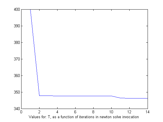
For log files generated by FMIT:
% FMIT generates logs in .txt format. Supply these to LogViewer which will
% extract the XML data present in them.
LogViewer('twoEqSteadyState_log.txt');
% LogViewer will create a new file, typically names 'twoEqSteadyState_log_extracted.xml'
% in this case and load it as well.
Creating Custom Problem Class (MATLAB)
It is also possible to implement subclasses to the Problem class. Below, a complete class TestProblem which is a subclass of Problem is given.
% Solving:
% FX = if(x < -1)
%         x + (x+1)*COEFF;
%      else
%         if(x > 1)
%             x + (x - 1)*COEFF;
%      else
%          x;
%      FX, COEFF defined below, INITX - initial X
classdef TestProblem < oct.nlesol.Problem

    properties (Access = public)
        sw0;
        sw1;
        COEFF = 2;
        FX = 2;
    end

    methods(Access = public)
        function this = TestProblem()
            this.sw0 = false;
            this.sw1 = false;
        end

        function [numberOfIterationVariables] = getNumberOfIterationVariables(this)
            numberOfIterationVariables = 1;
        end

        function [numDiscontinuities] = getNumberOfDiscontinuities(this)
            numDiscontinuities = 2;
        end

        function [indicators] = evaluateDiscontinuityIndicators(this, x)
            indicators = [-x - 1; x - 1 ];
        end

        function [residual] = evaluateResiduals(this, x)
            if(this.sw0)
                v = x + (x + 1)*this.COEFF;
            elseif(this.sw1)
                v = x + (x - 1)*this.COEFF;
            else
                v = x;
            end
            residual = this.FX - v;
        end

        function [xInitial] = getInitialGuess(this)
            xInitial = 2;
        end

        function makeDiscontinuousChange(this, x)
            this.sw0 = (x < -1);
            this.sw1 = (x > 1);
        end
    end
end
This class can then be sent to the solver in much the same manner as above:
import oct.nlesol.*; % Import nlesol package.
testProblem = TestProblem();
solver = Solver(testProblem);
solution = solver.solve()
Hold Iteration Variables (MATLAB)
This example shows how the hold iteration variable functionality works for FMUProblem. It uses the model from Interactive FMU, which is included in the ExampleModels.mo-package. The MATLAB® script to run this example is example_HoldIVs.m.
% The FMUProblem in this example contains two iteration variables. Using
% printInfo its structure is shown:

fmuProblem.printInfo()
:::::::: Iteration variables ::::::::
    1: 4.0000000000000000E+02 T
    2: 1.0000000000000000E+00 x
:::::::: Residual equations ::::::::
    1: -6.2700000000000000E+02 0 = (- x) * (873 - T) + 11.0 * (T - 300)
    2: -1.2000000000000000E+02 LongEq

% To hold an iteration variable the method "holdIterationVariables" is
% provided. Let's hold variable T
fmuProblem.holdIterationVariables([1])
% We could also use {'T'} as an argument

% Using printInfo again we see that T, and the corresponding residual
% equation is removed.
fmuProblem.printInfo()
:::::::: Iteration variables ::::::::
    2: 1.0000000000000000E+00 x
:::::::: Residual equations ::::::::
    2: -1.2000000000000000E+02 LongEq

% To restore the system we can use the method "releaseIterationVariables"
fmuProblem.releaseIterationVariables([1])

fmuProblem.printInfo()
:::::::: Iteration variables ::::::::
    1: 4.0000000000000000E+02 T
    2: 1.0000000000000000E+00 x
:::::::: Residual equations ::::::::
    1: -6.2700000000000000E+02 0 = (- x) * (873 - T) + 11.0 * (T - 300)
    2: -1.2000000000000000E+02 LongEq

% We can specify which residual equations that should be removed

fmuProblem.holdIterationVariables([2], [1]) % Remove x, and res. eq 1
fmuProblem.printInfo()
:::::::: Iteration variables ::::::::
    1: 4.0000000000000000E+02 T
:::::::: Residual equations ::::::::
    2: -1.2000000000000000E+02 LongEq

% Most methods on FMUProblem also lets you specify if you want to apply the
% method for active, held or all variables. Default is active.

fmuProblem.printInfo('held')
:::::::: Iteration variables ::::::::
    2: 1.0000000000000000E+00 x
:::::::: Residual equations ::::::::
    1: -6.2700000000000000E+02 0 = (- x) * (873 - T) + 11.0 * (T - 300)

fmuProblem.printInfo('all')
:::::::: Iteration variables ::::::::
    1: 4.0000000000000000E+02 T
    2: 1.0000000000000000E+00 x
:::::::: Residual equations ::::::::
    1: -6.2700000000000000E+02 0 = (- x) * (873 - T) + 11.0 * (T - 300)
    2: -1.2000000000000000E+02 LongEq

% It also possible change min/max/nominal attributes on the iteration
% variables. This can e.g. be used if the initial guess is close
% to the solution, where tighter bounds provides additional
% guidance to the solver. This may be particularly useful in case of
% multiple solutions.
Parametric Hold Iteration Variables (MATLAB)
In addition to manually held variables, there is functionality for setting up hold specifications based on parameters on the FMU. The Modelica compiler provided by OCT supports special annotations for marking variables for parametric holding, see Specification of Hand Guided Tearingfor a complete specification. The basic methodology behind parametric holding is that iteration variables and residuals are bound to boolean parameters. When the problem is constructed, the variables and residuals bound to boolean parameters that are true are automatically held. The model for this example is included in the ExampleModels.mo-package and the script to run the example is example_ParametricHoldIV.mo. In the model, parameters for parametric holding are specified for the iteration variables and residuals as follows:
model twoEqSteadyStateParaHold
    Real x (start = 1);
    Real T (start = 400);
    parameter Boolean testHold1 = false;
    parameter Boolean testHold2 = false;
equation
    0 = 120*x - 75*(0.12*exp(12581*(T - 298)/(298*T)))*(1 - x)
        annotation(__Modelon(ResidualEquation(hold = testHold1,
            iterationVariable(hold = testHold2)=x), name = LongEq));
    0 = -x*(873 - T) + 11.0*(T - 300)
        annotation(__Modelon(ResidualEquation(hold = testHold2,
            iterationVariable(hold = testHold1)=T), name = LongEq2));
end twoEqSteadyStateParaHold;
This model could be used to set up parametric holding:
fmu = loadFMU(fmuName);
fmu.setValue('testHold1', true);
fmuProblem = FMUProblem(fmu);

% Print the active variables - notice that an iteration/residual
% pair is held
fmuProblem.printInfo()
:::::::: Iteration variables ::::::::
    2: 1.0000000000000000E+00 x
:::::::: Residual equations ::::::::
    1: -6.2700000000000000E+02 LongEq2

% Print the parametrically held variables
fmuProblem.printInfo('parametricHold')
:::::::: Iteration variables ::::::::
    1: 4.0000000000000000E+02 T
:::::::: Residual equations ::::::::
    2: -1.2000000000000000E+02 LongEq
Parametric Start Attributes (MATLAB)
If the iteration variables were automatically found as part of the call to the constructor of FMUProblem, then the initial guess for all iteration variables that have start values that depend on a parametric expression will be altered. The parametric expression will be evaluated and the value set as the initial guess for all such variables.
It is possible to bypass this behavior and to set the initial guess explicitly if the values are set on the FMU followed by initialization of the FMU before it is passed as an argument to the constructor.
The model for this example is included in the ExampleModels.mo-package and the script to run the example is example_ParametricStart.m. In the model, one of the iteration variables has a parametric expression in its start value:
model twoEqSteadyStateParaStart
    parameter Real x_start = 1;
    Real x (start = x_start);
    Real T (start = 400);
equation
    0 = 120*x - 75*(0.12*exp(12581*(T - 298)/(298*T)))*(1 - x)
        annotation(__Modelon(ResidualEquation(iterationVariable=x)));
    0 = -x*(873 - T) + 11.0*(T - 300)
        annotation(__Modelon(ResidualEquation(iterationVariable=T)));
end twoEqSteadyStateParaStart;
This model would have the initial guess for x altered as part of the call to the constructor of FMUProblem:
% Change initial guesses for the iteration variables. The
% variables whose start values are not determined by a
% parameteric are not changed directly since FMU not initialized before
% call to FMUProblem constructor. Fixed start values will be used if there
% are any, otherwise parametric.
fmu = loadFMU(fmuName);
fmu.setValue('x_start', 10); % This will change guess for x
fmu.setValue('T', 20); % This will not change guess for T
fmuProblem = FMUProblem(fmu);

fmu.getValue('x')
10
fmu.getValue('T')
400

% Change initial guesses for the iteration variables. The
% variables whose start values are set as parameteric are not
% changed directly since fmu initialized
fmu = loadFMU(fmuName);
fmu.setValue('x_start', 10); % This will not change guess for x
fmu.setValue('T', 20); % This will change guess for T
fmu.fmiInitialize();
fmuProblem = FMUProblem(fmu);
fmu.getValue('x')
1
fmu.getValue('T')
20

% If the value of an iteration variable with a parametric start
% expression is explicitly set it will not be used since fmu not initialized:
fmu = loadFMU(fmuName);
fmu.setValue('x', 10); % This will not change guess for IterVar1
fmuProblem = FMUProblem(fmu);
fmu.getValue('x')
1

% However, if fmiInitialize was called before instantiation of the FMUProblem
% then the behavior would be bypassed and the above would work.
fmu = loadFMU(fmuName);
fmu.setValue('x', 10);
fmu.fmiInitialize(); % Bypass parameteric start behavior
fmuProblem = FMUProblem(fmu);
fmu.getValue('x')
10

% The same holds if the FMUProblem constructor is called with the
% argument pair ('guesses', 'interactive').
fmu = loadFMU(fmuName);
fmu.setValue('x', 10);
fmuProblem = FMUProblem(fmu, 'guesses', 'interactive');
fmu.getValue('x')
10

% No initialization but FMUProblem interactive
fmu = loadFMU(fmuName);
fmu.setValue('x_start', 10); % This will not change guess for x
fmuProblem = FMUProblem(fmu, 'guesses', 'interactive');
fmu.getValue('x')
1
fmu.getValue('T')
400

% Initialization but FMUProblem parametric, change of x_start has effect
% since GUESS_KIND set to 'parametric'
fmu = loadFMU(fmuName);
fmu.setValue('x_start', 10); % This will change guess for x
fmu.fmiInitialize();
fmuProblem = FMUProblem(fmu, 'guesses', 'parametric');
fmu.getValue('x')
10
fmu.getValue('T')
400
Steady-state Modelica Modeling with Hand Guided Tearing🔗
In the Optimica Compiler Toolkit, there are extensions to the Modelica language which give the possibilities to utilize hand-guided tearing. With hand-guided tearing the user can specify certain variables and equations which should be chosen as iteration variables and residuals respectively. Normally this choice is made automatically by the compiler. In this Chapter, the syntax and the method will be explained.
Specification of Hand-Guided Tearing🔗
There are two ways to use hand-guided tearing in OCT:
• As pairing where an equation is bound to a variable
• As unpaired variables and equations where pairs are bound by the compiler
Identification of Equations🔗
In some situations, it is necessary to identify an equation so that it can be referenced.
Syntax
"annotation" "("
  "__Modelon" "("
    "name" "=" IDENT
  ")"
")"
Example
x = y + 1 annotation(__Modelon(name=res));
Paired Tearing🔗
In some situations, it is crucial that an equation and a variable form a tearing pair. This is where the hand-guided tearing pair annotations come into play. It allows the user to specify exactly which tearing pairs to form. The tearing pairs that are specified are torn before any automatic tearing comes into play. The pairs are also torn without any regard for the solvability of the system. This means that if the user specifies too many pairs, they will all be used and the torn block becomes unnecessarily complex. If the final system is unsolvable after all pairs are torn, the automatic algorithm will kick in and finalize the tearing.
There are two ways to specify hand-guided tearing pairs.
• On the component level
• On the system level
Specify Tearing Pairs on the Component Level🔗
Tearing pairs can be specified in the annotation for the equation that should become the residual equation. This type of hand-guided tearing is limited to the name scope that is visible from the equation. In other words, the equation has to be able to "see" the variable that should be used as an iteration variable.
Syntax
It is possible to place annotations for tearing pairs in the annotation block for the residual equation. The syntax for tearing pair on the component level has the following syntax:
"annotation" "("
  "__Modelon" "("
    ResidualEquation
  ")"
")"
Where ResidualEquation is defined by the following record declaration:
record ResidualEquation
  parameter Boolean enabled = true;
  parameter Integer level(min=1) = 1;
  Real nominal = 1;
  IterationVariable iterationVariable;
  parameter Boolean hold = false;
end ResidualEquation;
Where IterationVariable is defined by the following record declaration:
record IterationVariable
  parameter Real name; // Accessed without dot-notation
  Real max;
  Real min;
  Real nominal;
  Real start;
  parameter Boolean hold = false;
end IterationVariable;
Example
model A
  ...
  parameter Boolean subSystem1Hold = true;
  Real z;
  Real q;
  ...
equation
  ...
  x = y + 1 annotation(__Modelon(ResidualEquation(iterationVariable=z)));

  p = x + q annotation(__Modelon(ResidualEquation(
                                   iterationVariable(
                                     start = 1,
                                     nominal = 10,
                                     hold = subSystem1Hold
                                    ) = q,
                                    nominal = 100,
                                    hold = subSystem1Hold,
                                )));
 ...
end A;
Specify Tearing Pairs on the System Level🔗
Tearing pairs on the system level is necessary when the residual equation and iteration variable are located in different name scopes. In other words, the equation can not "see" the iteration variable.
Before it is possible to specify tearing pairs on the system level it is necessary to define a way to identify equations.
Syntax
It is possible to place annotations for tearing pairs on the system level in the annotation block for the class deceleration.
"annotation" "("
  "__Modelon" "("
    "tearingPairs" "(" Pair* ")"
  ")"
")"
Where Pair is defined by the following record declaration:
record Pair
  parameter Boolean enabled = true;
  parameter Integer level(min=1) = 1;
  ResidualEquation residualEquation;
  IterationVariable iterationVariable;
end Pair;
Where ResidualEquation is defined by the following record declaration:
record ResidualEquation
  parameter Equation name; // Accessed without dot-notation
  Real nominal = 1;
  parameter Boolean hold = false;
end ResidualEquation;
Where IterationVariable is equal to the record declaration with the same name in Specify Tearing Pairs on Component Level:
Example
Here follows an example where the equation is identified by a name tag and then paired with a variable.
Model A
  model B
    ...
    x = y + 1 annotation(__Modelon(name=res));

    p = x + q annotation(__Modelon(name=res2));
    ...
  end B;
  model C
    ...
    Real z;
    Real q;
    ...
  end C;
  parameter Boolean subSystem2Hold = true;
  B b;
  C c;
  ...
  annotation(__Modelon(tearingPairs(Pair(residualEquation=b.res,iterationVariable=c.z))));

  annotation(__Modelon(tearingPairs(Pair(
                         residualEquation(
                           nominal = 10,
                           hold = subSystem2Hold
                         ) = b.res2,
                         iterationVariable(
                           start = 2,
                           hold = subSystem2Hold
                         ) = c.q
                       ))));
end A;
Unpaired Tearing🔗
It is also possible to specify that an equation or variable should be used in tearing without pairing. This is useful when there is no requirement that a certain equation is bound to a specific variable. The pairing is instead done by the compiler during compilation. An error is given If the number of unpaired equations is unequal to the number of unpaired variables.
Specify an Equation as an Unpaired Residual Equation🔗
By marking an equation as an unpaired residual equation it will be paired with an unpaired iteration variable during tearing.
Syntax
It is possible to place annotations for residual equations in the annotation block for an equation. The syntax for residual equation annotation has the following syntax:
"annotation" "("
  "__Modelon" "("
    ResidualEquation
  ")"
")"
Where ResidualEquation is equal to that of component level pairs (see Specify Tearing Pairs on Component Level) with one exception; the iterationVariable field is left unspecified.
Example
x = y + 1 annotation(__Modelon(ResidualEquation));
Specify a Variable as an Unpaired Iteration Variable🔗
By marking a variable as an unpaired iteration variable it will be paired with an unpaired residual equation during tearing.
Syntax
It is possible to place annotations for unpaired iteration variables in the annotation block for a variable. The iteration variable annotation has the following syntax:
"annotation" "("
  "__Modelon" "("
    IterationVariable
  ")"
")"
Where IterationVariable is defined by the following record declaration:
record IterationVariable
  parameter Boolean enabled = true;
  parameter Integer level(min=1) = 1;
  Real max;
  Real min;
  Real nominal;
  Real start;
  parameter Boolean hold = false;
end IterationVariable;
Example
Real x annotation(__Modelon(IterationVariable));
Nested Hand Guided Tearing🔗
The record definitions ResidualEquation and IterationVariable in Specification of Hand Guided Tearing have the field declaration level. This field specifies on which level the equation or variable should be torn. Equations and variables with the same level will be torn into the same torn block. It is possible to have nested torn blocks by specifying different levels for different equations and variables.
Hand-Guided Tearing Attributes🔗
The record definitions ResidualEquation and IterationVariable in Specification of Hand Guided Tearing have the field declarations max, min, start and nominal. These fields are optional. If left unspecified, the value is retrieved from the corresponding attributes in the variable declaration specified by the name field. It is possible to use continuous variables in the expressions for the fields max, min, nominal, start and equation nominal with two restrictions; the variable must be solved before the computation of the equation block start and the block must be torn on HGT level two or greater.
Extended Example🔗
NHGT with fixed bounds🔗
Consider the following two-dimensional nonlinear algebraic test problem. It depends on two unknowns x1 and x2. The first residual equation is

It involves a sub-expression.

The second residual equation is

Again, sub-expressions are used.

The shape of the residuals is as follows (the first residual is blue, the second green, and black lines illustrate the intersection with the zero plane). Note how the blue residual is non-convex. This means that a gradient-based algorithm will have difficulties to reach the solution inside the “valley” for small x1 values unless the algorithm is started inside (i.e., the start attributes correspond to an iterate inside the “valley”).
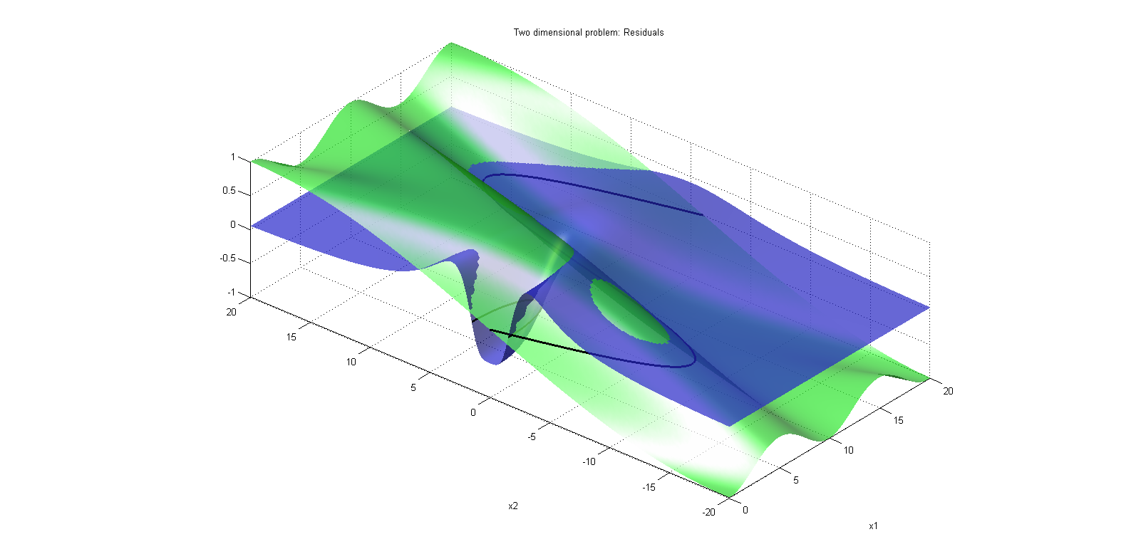
The Modelica code for such a model can be written as follows. This model is included in the ExampleModels.mo-package and the script to run this example is example_NHGT.
model NonConvex
  import Modelica.Math.*;
  import Modelica.Constants.pi;
  Real r;
  Real a;
  Real b;
  Real x1(min=0, max=20, start=15);
  Real x2(min=-20, max=20, start=15);
equation
  r = x1^2/100+x2^2/10;
  0 = 3*exp(-1/(r+0.1))/(r+0.1)-1/(r+2);
  a = pi*x2/40;
  b = sin(x1/pi);
  0 = sin(a + b);
end NonConvex;
How can we solve such a problem using nested hand-guided tearing, ideally such that the robustness is high? We split the problem into two levels. On the inner level (“level 2”), the solver finds the solution x2 to the second residual based on the current iterate of x1. In other words, the solver iterates are constrained to the following one- dimensional manifold (see the black line in the following illustration).
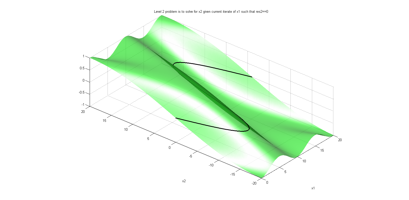
To achieve this, we add a nested hand-guided tearing annotation to the residuals equation as described in the introductory section (see bold text).
model NonConvex
  import Modelica.Math.*;
  import Modelica.Constants.pi;
  Real r;
  Real a;
  Real b;
  Real x1(min=0, max=20, start=15);
  Real x2(min=-20, max=20, start=15);
equation
  r = x1^2/100+x2^2/10;
  0 = 3*exp(-1/(r+0.1))/(r+0.1)-1/(r+2);
  a = pi*x2/40;
  b = sin(x1/pi);
  0 = sin(a + b)
    annotation(__Modelon(ResidualEquation(iterationVariable=x2,level=2)));
end NonConvex;
Finally, in the outer “level 1” problem, the solver drives the first residual to zero. This problem can be solved robustly (i.e., without suffering from the non-convex shape of the residual) using a computationally efficient algorithm. The algorithm moves along the same one-dimensional manifold highlighted with a black line in the following illustration. Residual 1 is evaluated along this manifold, and a solution is computed.
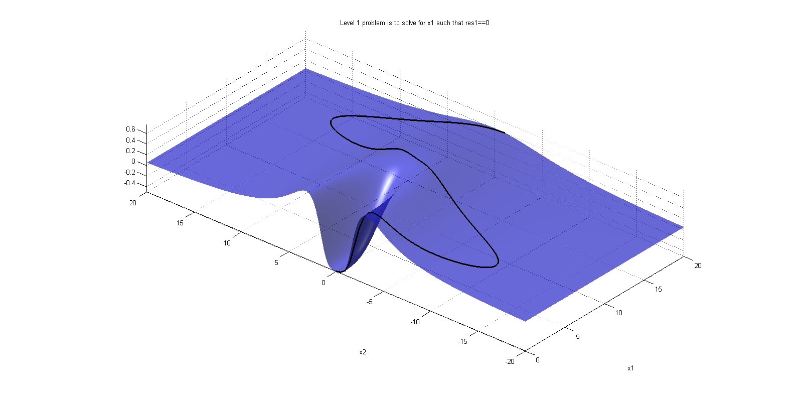
This is implemented via the following additional annotation (again, see the bold text). The model with these annotations is also included in the ExampleModels.mo-package.
model NonConvexNHGT
  import Modelica.Math.*;
  import Modelica.Constants.pi;
  Real r;
  Real a;
  Real b;
  Real x1(min=0, max=20, start=15);
  Real x2(min=-20, max=20, start=15);
equation
  r = x1^2/100+x2^2/10;
  0 = 3*exp(-1/(r+0.1))/(r+0.1)-1/(r+2)
    annotation(__Modelon(ResidualEquation(iterationVariable=x1,level=1)));
  a = pi*x2/40;
  b = sin(x1/pi);
  0 = sin(a + b)
    annotation(__Modelon(ResidualEquation(iterationVariable=x2,level=2)));
end NonConvexNHGT;
In the compilation log files, we get the following visualization of the problem structure.
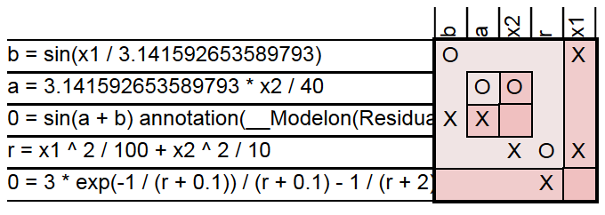
NHGT with adaptive bounds🔗
Additionally to allowing to the modeler to specify in what hierarchy to solve an equation system, Nested Hand Guided Tearing allows to adapt Real variable attributes such as the start value. Consider the following two-dimensional problem. The residual equations are

The equation system involves three further equations (and unknowns k, l, s), which we will ask the compiler to solve for as needed to express the problem in terms of two residuals. The variable f is a problem-specific parameter.

Substituting the three equations as required into the two residual equations, we can visualize the problem as follows (again, the blue surface is the first and the green surface is the second residual). Note how the blue residual admits two one-dimensional manifolds to satisfy it.
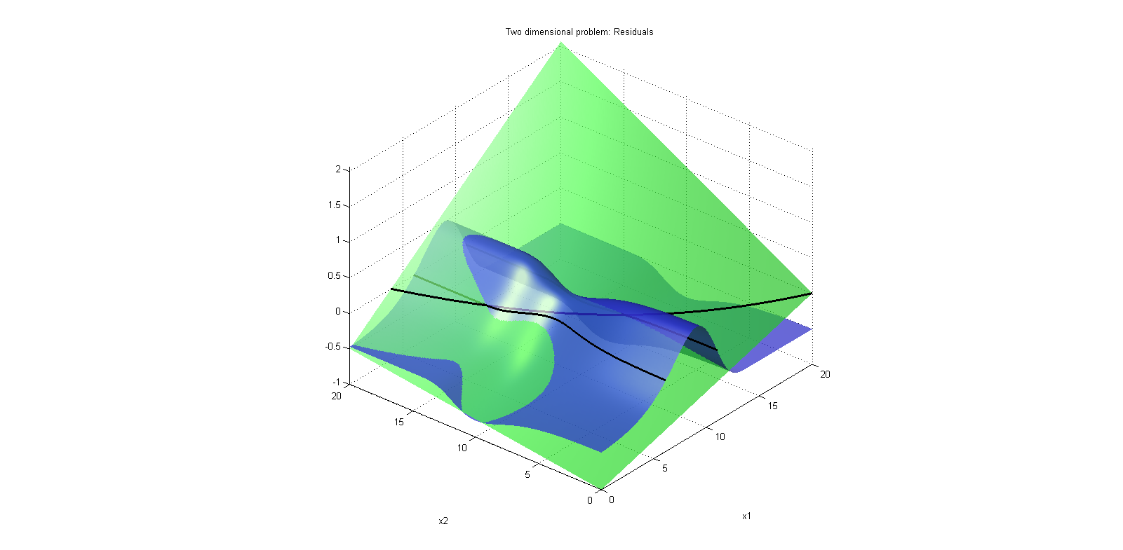
Without Hand Guided Tearing we formulate this problem in Modelica as follows.
model Test
  parameter Real f = 10;
  Real x1(min=0, max=20, start=15);
  Real x2(min=0, max=20, start=15);
  Real k;
  Real l;
  Real s;
equation
  0 = k +(x1-9)/(-2);
  0 = l +(x2-f)/(-2);
  0 = x2/40 + x1/20 - s;
  0 = 1 * exp(-exp(k)+k+1.0) - 0.3 * exp(-exp(l)+l+1.0) - 0.5;
  0 = s + x1*x2/16^2 - 1;
end Test;
Assume that, based on an understanding of the problem (usually given its physics-based characteristics of it), we can infer that solving residual two in a nested fashion is particularly beneficial for robustness or computational efficiency. The “level 2” problem shall be to solve residual two for x2 given the current iterate of x1. In the following illustration, the one-dimensional manifold is shown as a black line.
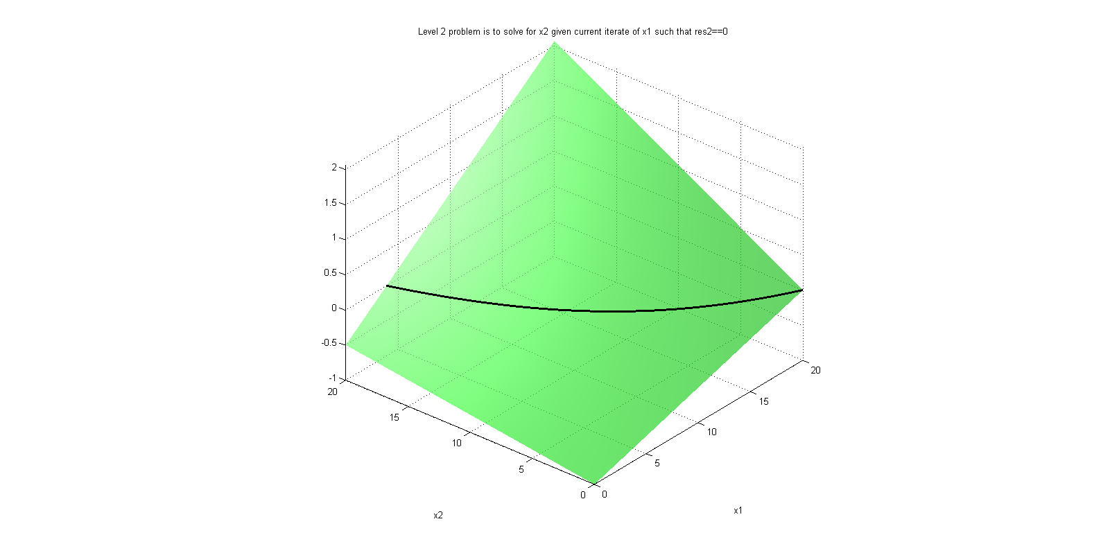
The “level 1” problem is now to vary variable x1 until the problem is solved. Again, the algorithm moves along the same one-dimensional manifold highlighted with a black line in the following residual 1 illustration.
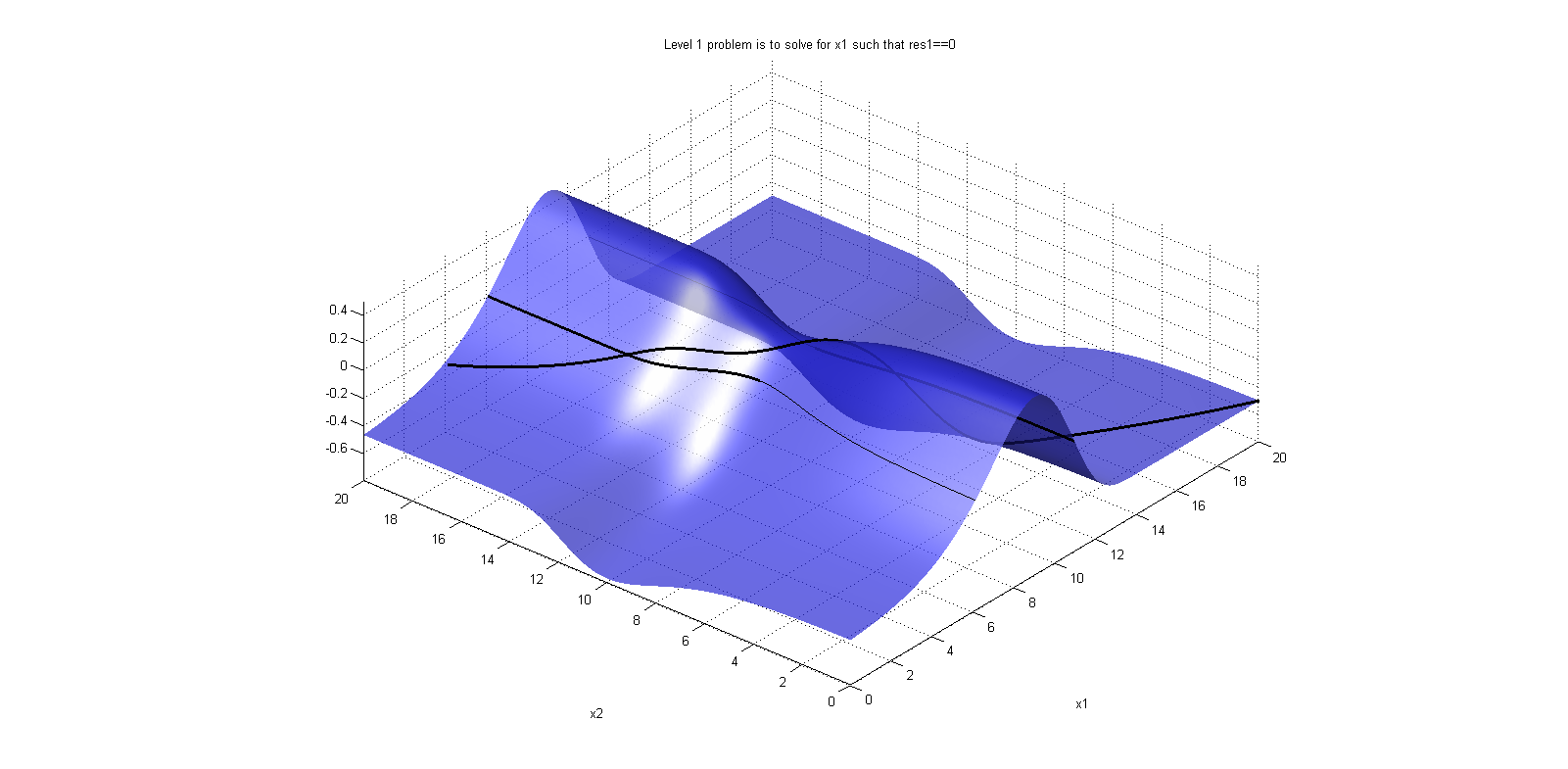
These two different levels can be implemented with the following annotations (see text in bold font).
model Test
  parameter Real f = 10;
  Real x1(min=0, max=20, start=15);
  Real x2(min=0, max=20, start=15);
  Real k;
  Real l;
  Real s;
equation
  0 = k +(x1-9)/(-2);
  0 = l +(x2-f)/(-2);
  0 = x2/40 + x1/20 - s;
  0 = 1 * exp(-exp(k)+k+1.0) - 0.3 * exp(-exp(l)+l+1.0) - 0.5
    annotation(__Modelon(ResidualEquation(iterationVariable=x1,level=1)));
  0 = s + x1*x2/16^2 - 1
    annotation(__Modelon(ResidualEquation(iterationVariable=x2,level=2)));
end Test;
This problem does however exhibit two different solutions. In engineering, one of the multiple solutions is usually superior if compared to the others. In some cases, the solutions differ in efficiency or a similar metric, in others some of the solutions may even be mathematical artifacts that are not physically possible (because they violate fundamental laws such as the Second Law of Thermodynamics). We assume that a condition can be written to express such a condition, and, based on its value, the attributes of the real iteration variables are adopted.
In this simple example, we assume that any solution with x1 + x2 > 20 can be excluded based on physical insight. We, therefore introduce an adaptive bound on the “level 2” problem by setting the lower bound to x2, max = 20 - x1. This condition is illustrated below with the grey transparent surface; all points facing the reader “before the surface” are valid.
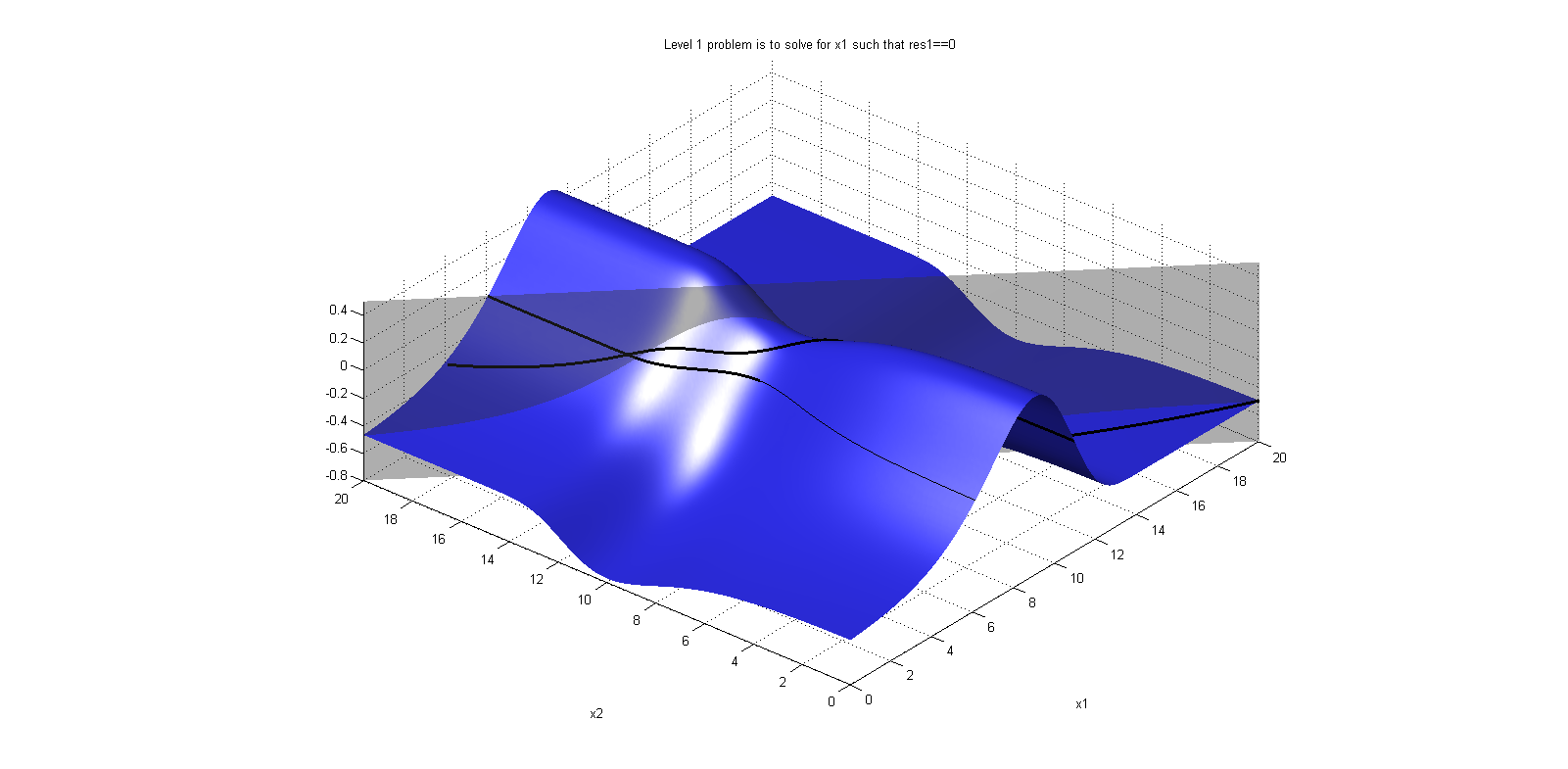
These adaptive bounds are implemented as follows.
model Test
  parameter Real f = 10;
  Real x1(min=0, max=20, start=15);
  Real x2(min=0, max=20, start=15);
  Real k;
  Real l;
  Real s;
equation
  0 = k +(x1-9)/(-2);
  0 = l +(x2-f)/(-2);
  0 = x2/40 + x1/20 - s;
  0 = 1 * exp(-exp(k)+k+1.0) - 0.3 * exp(-exp(l)+l+1.0) - 0.5
    annotation(__Modelon(ResidualEquation(iterationVariable=x1,level=1)));
  0 = s + x1*x2/16^2 - 1
    annotation(__Modelon(ResidualEquation(iterationVariable(max=20-x1)=x2,level=2)));
end Test;
The compilation log again contains a visualization of the equation structure with the BLT table.
Bibliography🔗
[Mag2015] Fredrik Magnusson and Johan Åkesson. Dynamic Optimization in JModelica.org. 471-496. Processes. 3:2. 2015.
[Mag2016] Fredrik Magnusson. Numerical and Symbolic Methods for Dynamic Optimization. Lund University. Sweden. 2016.
Resources🔗
Send an email ![]() to support@modelon.com for OPTIMICA Compiler Toolkit User's guide.
to support@modelon.com for OPTIMICA Compiler Toolkit User's guide.