Refueling🔗
In this section, we continue from the Sizing Tutorial to test the tanks that were sized with different filling rates.
Base Class setup to test🔗
Now that we have the tank geometric parameters, we’ll test them in 3 scenarios: Filling, Storage and Extraction. Many of the components and parameters will be the same for all experiments, so we’ll create a base class to reuse instead of building each test model from scratch.
-
Create a new package in the workspace as Workspace.Experiment and inside add a new model named TankTestBase.
-
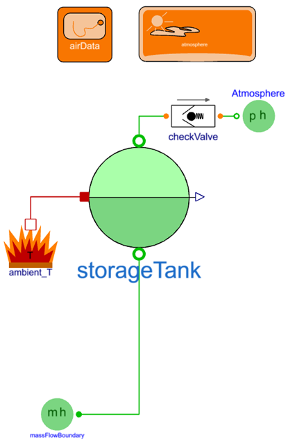
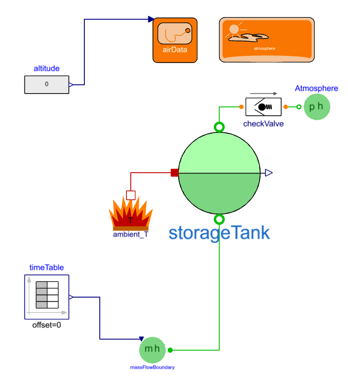
Instantiate and connect the following components:
- Modelon.ThermoFluid.Volumes.TwoPhaseTankSimpleWall as storageTank
- The parameter enable_externalHeatPort needs to be set true to enable the thermal port for the tank.
- Modelon.ThermoFluid.Valves.CheckValve as checkValve.
- VaporCycle.Sources.TwoPhasePressureSource as Atmosphere.
- VaporCycle.Sources.TwoPhaseFlowSource as massFlowBoundary.
- Modelon.ThermoFluid.Sources.Environment_T as ambient_T.
- Modelon.Environment.AtmosphereImplementations.ISA (note: atmosphere name is added automatically which should not be changed).
- Modelon.Environment.AirDataImplementations.XYZ (note: airData name is added automatically which should not be changed).
- Modelon.ThermoFluid.Volumes.TwoPhaseTankSimpleWall as storageTank
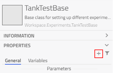
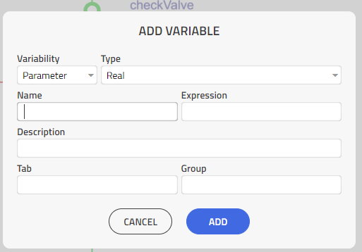
- Declare parameters – To make it easier to setup the different experiments, we’ll declare parameters that are used to compute intermediate parameters and propagate them to the components in this base class. Use the ADD VARIABLE interface found in the right-side panel in the PROPERTIES section. The Type can be filtered by typing in the unit of interest.
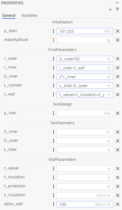
Create the parameters and enter the corresponding values from the table,
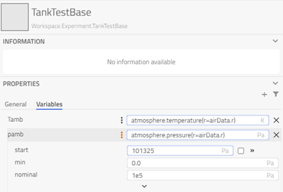
- Variables – Ambient temperature and pressure are inputs that vary based on the altitude. They’re calculated using a function from the atmosphere model that was instantiated based on the position “r” from the airData block, which will be used later to specify altitude.
| Type (Modelica.Units.SI) | Name | Expression | Description |
|---|---|---|---|
| Modelica.Units.SI.Temperature | Tamb | atmosphere.temperature(r=airData.r) | Ambient temperature |
| Modelica.Units.SI.AbsolutePressure | pamb | atmosphere.pressure(r=airData.r) | Ambient pressure |
- For pamb, in the parameter panel, click on the three-dots icon to access the modifiers and give a start value of 101325 Pa so that it does not initialize with the default value of zero.
The tank initialization can be specified by liquid level, volume or mass. We want to be able to initialize based on mass, so the volume needs to be calculated at initialization tab (group: Liquid level) to initFromMass. This enables the parameter M_tot_start which should be assigned to massHydAvail. The necessary liquid-level at initialization is then computed based on the given inputs and known liquid and vapor densities.
-
Start the propagation of parameters to components.
-
airData:
- alt_input = true (to provide the altitude with an input signal).
-
massFlowBoundary:
- Set the Medium as VaporCycle.Media.Naturals.HydrogenMbwr
- Set use_m_flow_in as true, so that a dynamic source can be connected as an input.
- Change the energyInput to be defined by Temperature and set T = 20 K, which will be assumed to be the source temperature for hydrogen when the tank is being filled.
-
ambient_T:
- T0 = Tamb (The temperature calculated from the atmosphere model and altitude.)
-
storageTank:
- Set the Medium as VaporCycle.Media.Naturals.HydrogenMbwr
- Now to the right of the drop-down list there will be a paint bucket icon
 to ‘Propagate’. Click on this so that the connected components will also redeclare their Medium to match the storageTank.
 -
Set the geo as HorizontalCylinderEllipsoid and set:
- r_internal = r_inner, the internal radius of the cylinder.
- s_end = r_inner, the distance from the cylindrical section to the ends of the hemispherical end caps.
- L = L_cylinder, the length of the cylindrical section.
- t_wall = t_insulation, the thickness of the wall being considered for thermal insulation. The vessel and protection layer have a higher relative thermal conductivity, so they’re ignored.
Note
The storageTank.t_wall is a parameter within this component, and the t_wall mentioned in table is a top-level parameter of the model TankTestBase.
- Check that enable_externalHeatPort = true to connect to the Environment_T component.
- Redeclare the internalConvection model to ConstantCoefficient, where the alpha_dry_prescribed and the alpha_wet_prescribed are set to fill(alpha_wall,2).
- K_cond_surface = 1e-3, condensation coefficient at liquid/vapor interface.
- g_surface = 4 W/(m2K), heat transfer coefficient at liquid/vapor interface.
- g_external = k_insulation/t_insulation, heat transfer coefficient between the tank wall and exterior.
- k_wall = k_insulation, the thermal conductivity of the tank wall.
-
Within the Properties section, navigate to the Initialization tab:
- p_start = p_start, initial pressure in the tank.
- Check that tankInitQuantity = initFromMass, so we can initialize from initial hydrogen mass.
- M_tot_start = massHydAvail, initial mas of hydrogen in the tank.
-
checkValve:
- zeta_A = 0.1, loss factor for flow.
- A_open = 1e-4, the cross-sectional area for the fully opened valve.
- dp_open = p_max – 101305 Pa, the pressure difference at which the valve is completely opened.
- dp_closed = checkValve.dp_open – 10000 Pa, the pressure difference at which the valve is completely closed.
- relativeOpening_start = 0, to start closed.
-
Atmosphere:
- p = pamb, the pressure boundary based on the atmosphere model using airData position.
- energyInput = Temperature, to define by temperature rather than the enthalpy.
- T = Tamb, the temperature determined from the atmosphere model.
-
-
The base class is complete. The key parameters are accessible from the top-level of the model in the parameter dialog and propagate the required information to each component. To set up experiments, signals need to be supplied to the airData.alt_in and massFlowBoundary.m_flow_in inputs and values assigned to parameters with no default.
Filling Experiment🔗
This section observes the temperature and pressure evolution in the tank during a refueling scenario. Using the base class from the previous section, boundary conditions are imposed and experiments are set up to compare the effects of different refueling mass flow rates.
Overview🔗
- Setup system boundaries.
- Define Experiments for Foam and Vacuum.
- Analyze tank conditions when filling the tank with hydrogen.
- Compare tanks and different fill rates.
System setup🔗
- Create a new model in the Experiments package by extending from the base class Workspace.Experiments.TankTestBase and call it TankFilling.
Note
Right-click on the class in the left pane to find the Extend… option from the context menu
-
Drag and drop in components to provide inputs to the airData and massFlowBoundary.
- Modelica.Blocks.Sources.RealExpression call it as altitude.
- Connect this to the alt_in connector for airData.
- Modelica.Blocks.Sources.TimeTable call it as timetable.
- Connect this to the m_flow_in connector of massFlowBoundary.
- Modelica.Blocks.Sources.RealExpression call it as altitude.
-
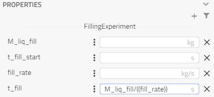
Add new parameters for the FillingExperiment:
- Modelica.Units.SI.Mass M_liq_fill, is the amount of fuel to transfer into storage tank.
- Modelica.Units.SI.Time t_fill_start, is the time at which to start filling the storage tank.
- Modelica.Units.SI.MassFlowRate fill_rate, is the he mass flow rate of filling.
- Modelica.Units.SI.Time t_fill = M_liq_fill / fill_rate, is the time it takes to fill the tank with M_liq_fill.
-
Parameterization of additional components:
- For altitude, keep y = 0 since the refueling is tested at ground level.
-
For timeTable, the table will create a ‘pulse’ with the magnitude fill_rate, starting at t_fill_start and with the duration of t_fill.
table = [0,0; t_fill_start,0; t_fill_start,fill_rate; t_fill_start + t_fill,fill_rate; t_fill_start + t_fill,0] -
For storageTank, change tankInitQuantity to initFromLevel and rel_level_start to 0.01 in the Initialization tab. We want to start from relatively empty, this will ensure that the tank is not too dry.
The basis of the filling experiment is now set up, but there are parameters still missing values, but they’ll be defined when setting up the Experiments.
Experiment: Foam 232🔗
-
Switch to Experiment mode and create a new Experiment named “Foam232”.
-
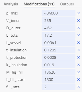
Enter the Foam232 variant geometry from the sizing model (values have been rounded).
| Parameter | Value |
|---|---|
| p_max | 404 kPa |
| V_inner | 235 m3 |
| D_outer | 4.67 m |
| L_total | 17.0 m |
| t_vessel | 0.00484 m |
| t_insulation | 0.117 m |
| t_protection | 0.0008 m |
| k_insulation | 0.015 W/(m K) |
- Enter test parameters
- The fill_rate can be between 0.1 – 20 kg/s** for low-pressure liquid hydrogen refueling between tanker trucks and LH2 aircraft tanks.
Note
massHydAvail is not being used because the storageTank is initializing with liquid level instead of mass.
| Parameter | Value |
|---|---|
| M_liq_fill | 13620 kg |
| t_fill_start | 1800 s |
| fill_rate | 2 kg/s |
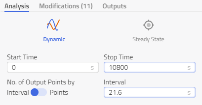
- Set the analysis mode to Dynamic with a Stop Time of 10,800 s and Interval to 21.6 s so that there are 500 points.
-
Simulate the experiment and then plot the results
-
Variables:
-
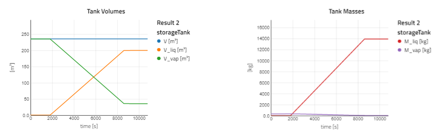
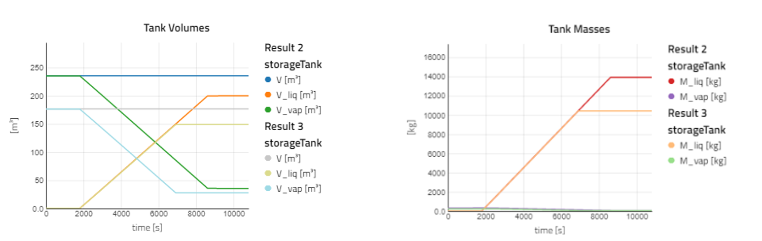
Filter with “storageTank.V” and plot V, V_liq and V_vap together. Rename the plot to Tank Volumes.
-
Filter with “storageTank.M” and plot M_liq and M_vap in their own plots. Rename the plots to Hydrogen Mass.
-
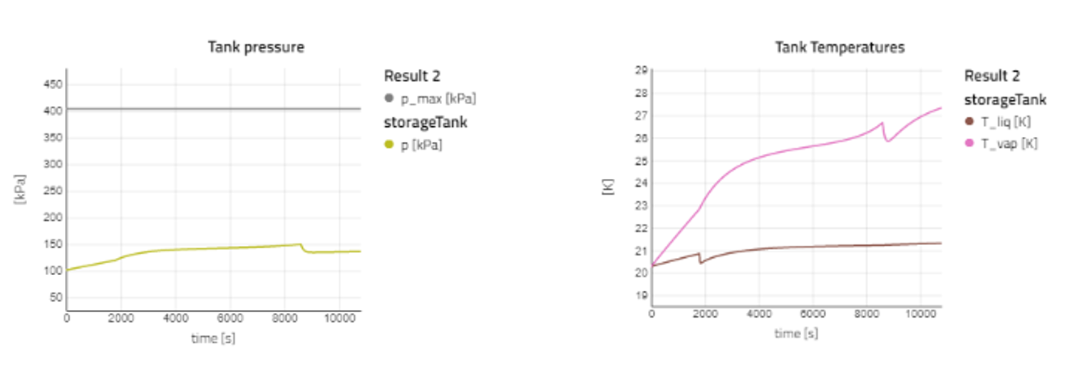
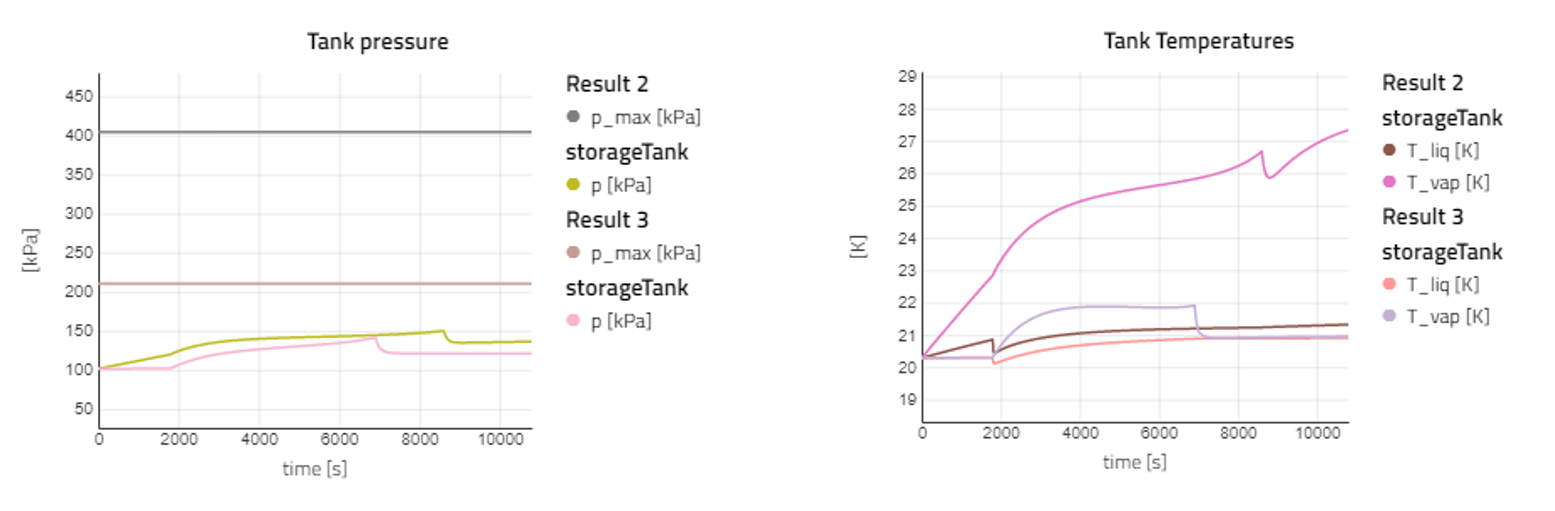
Filter with “storageTank.T” and plot T_liq and T_vap together. Rename the plot to Tank Temperatures.
-
Plot p_max with storageTank.p to check tank pressure.
-
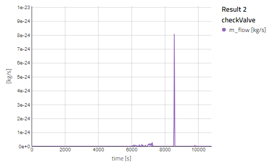
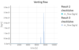
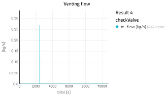
Plot checkValve.m_flow for the Vent off mass flow rate. Save the view as “Results” so it can be used later.
-
-
Experiment: MLI 232🔗
-
Switch to Experiment mode and create a new Experiment named “MLI232”.
-
Enter the MLI33 variant geometry.
| Parameter | Value |
|---|---|
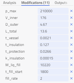
| p_max | 210 kPa |
| V_inner | 176 m3 |
| D_outer | 4.67 m |
| L_total | 13.6 m |
| t_vessel | 0.0033 m |
| t_insulation | 0.127 m |
| t_protection | 0.0265 m |
| k_insulation | 0.00015 W/(m K) |
- Enter test parameters.
| Parameter | Value |
|---|---|
| M_liq_fill | 10220 kg |
| t_fill_start | 1800 s |
| fill_rate | 2 kg/s |
- Set the analysis mode to Dynamic with a Stop Time of 10,800 s and Interval to 21.6 s so that there’s 500 points.
- Simulate the experiment and then activate the “Results” view. The results for both foam and MLI should be plotted together.
-
Observations
- With the plots its more noticeable that the Foam232 tank has a large volume since it takes more time to fill at the same rate and has more hydrogen mass at the end.
- Due to the heat ingress the liquid temperature raises after entering the tank, but also due to the pressure increase as well.
- The temperature of the vapor in the foam tank increases much more than the MLI due to the thermal conductivity of the foam being much higher.
- At this fill rate there are no concerns about excess pressure and needing to vent.
Experiment: MultiRate🔗
Let’s see at what fill_rate would cause pressures to rise too high.
-
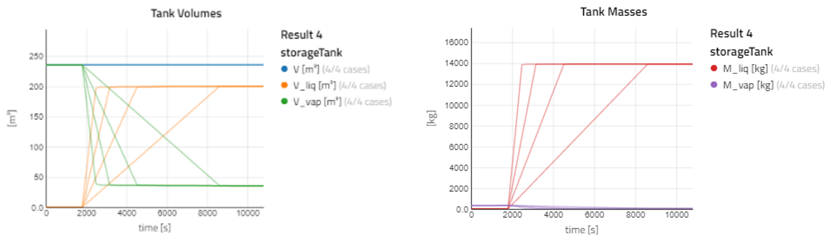
Duplicate the Foam232 experiment and name it as MultiRate, then set fill_rate = choices(2,5,10,20). This will simulate the experiment for each of the choices listed, making 4 cases.
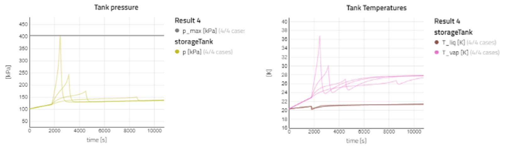
- At faster fill rates the temperature and pressure of the tank increases more.
- As the liquid level rises and the gas is compressed, the increased pressure increases the saturation temperature above the liquid temperature causing surface condensation.
- When either the filling stops or the checkValve opens to relieve the pressure, the rise of pressure and temperature stops and settles closer to the liquid temperature.
Suggestion🔗
-
Setup another experiment to observe how fill_rate affects the MLI tank.
-
What about refilling at different altitudes or ambient conditions?